Originally written August 2017 (English translation based on the original Hebrew version) – Updated May 2022 – Revised January, April, & November 2024; April & October-November 2025
Theory of Spheres' ('Quantum Gravity')'
or
'E'Empty Spheres in Dimensionless Space' – The 'Fundamental Force Behind Everything
(.Q('Quantum – Gravitational Force', 'Dark Matter' / 'Dark Energy', etc)
Eran Shimony (ORCID number – 0009-0003-5610-6736)
Physicist (B.Sc.), MBA, and Certified Real Estate Appraiser
i
Download the complete research papers in PDF format for offline reading and citation:
[Download Article I: The Framework (PDF)]
[Download Article II: The Spheres Classical components (PDF)]
[ Download Article III: The Quantum–Gravitational Force as Derived from the Spheres (PDF)]
[Paper III(a) – Updated version: The Quantum–Gravitational Force as Derived from the Spheres (PDF)]
[Download Article Ⅳ: The Planck's constant – ℏ (PDF)]
[Download Article VII: Introduction to the New Quantum Geometry Formalism (PDF))]
[Download Article IX: Introduction to the New Quantum Geometry Formalim (PDF))]
h
This article presents the English translation of the original Hebrew paper 'Theory of the Spheres', first published in its complete form in 2017. It proposes a 'Geometric—Quantum Model for Gravity' and related 'Cosmic Phenomena'.
Later published on December 29, 2025 (DOI: 10.5281/zenodo.18081185).
The empirical validation is presented in the subsequent work: 'Theory of Spheres – Part II', published on February 01, 2026 (DOI: 10.5281/zenodo.18446035)
i
ABSTRACT
The 'Theory of Spheres' (ToS) is introduced, built on the author's fundamental tenet of simplicity in nature. This comprehensive geometric-quantum model proposes that the universe is fundamentally constructed from discrete 'Near-Absolute Vacuum Points' (NAVPs/Spheres).
The theory successfully unifies General Relativity and Quantum Mechanics through a simple geometric principle, thereby eliminating the need for complex dimensions or string postulates. It explains gravity as derived from the outside pressure of these spheres, thereby eliminating the Einstein equation singularity and suggesting an exponentially decaying coefficient near the 'Event Horizon'/'Schwarzschild Radius'. Crucially, this same mechanism—deriving from the sphere’s internal movement—also accounts for Dark Energy and the Matter-Antimatter Asymmetry.
ToS extends a further standard framework by proposing the existence of an 'Entangled Quartet' of twin universes, which accounts for Dark Matter and suggests a physical basis for 'Color Charge' and for the Strong Nuclear Force, removing the requirement for gluons as mediating particles in specific contexts. Furthermore, ToS provides fundamental explanations for major observed phenomena: the Cosmic Microwave Background (CMB) temperature (2.7 K) is shown to be consistent with a state of near-absolute vacuum, and the Casimir Effect is explained as a direct result of the pressure differential exerted by the 'Spheres Quantity', superseding the concept of virtual particles.
The paper concludes by proposing a definitive Optical Experiment to test the theory's predictions on the speed of light changing over time. Furthermore, it provides a qualitative empirical explanation for the Hubble Tension, suggesting that the 5%-10% discrepancy in measurement is a direct consequence of the asymptotic nature of the expansion rate under a time-varying speed of light. Additionally, the paper highlights the Casimir Effect as existing empirical validation for the sphere's physical mechanism.
Part A: Introduction
From a very young age, I was occupied with the question of how the world around us was created and functions. A further question arose: Should the answer come, for me, from the realm of science or from the realm of religion 'God' / 'Higher Power')? In my search for answers, as a child, I attended enrichment programs in physics and astronomy at the Weizmann Institute of Science in Rehovot and at the Givatayim Observatory, and I devoured every Hebrew-language physics book I could find, including translations of Stephen Hawking's.
Later, before my military service, I explored the religious path. For several years, I participated in a course for returnees to religion, led by a rabbi who had himself returned to faith years earlier. After my military service, I also attended several lectures on Kabbalah. From these experiences, I concluded that although I did not receive a definitive answer regarding the existence or non-existence of God, the answer to how the world was created and how it works would not, for me, come from religion. I then decided to pursue a Bachelor's degree in physics at the Hebrew University.
During my academic studies, initially for personal reasons, I began drafting a short paper to address the question of the universe’s origin. Over time, after years of proposing and rejecting various ideas, the concept of the 'Spheres' emerged.
As I began writing the first chapters over twenty years ago, I encountered many contradictions that forced me to revise repeatedly. As the concept of the spheres solidified in its near-final form, it became clear that it contained apparent contradictions with some foundational assumptions of physics, such as the 'Constancy of the Speed of Light' and the 'Big Bang Theory' of the universe’s development.
It was only in 2017 that I completed the first version of the first part (B) of the paper, a version that has since been revised and expanded. Following feedback from friends and scientists, additional chapters were added. The paper now offers a 'Geometric Quantum Theory of Gravity' that seeks to 'Unify Gravitational Force with the Other Fundamental Forces of Nature', and a general theory about the structure of the universe, addressing its creation and evolution.
The 'Theory of Spheres' (ToS), beyond being a 'Theory of Quantum Gravity', also aims to explain other phenomena such as 'Dark Matter' and 'Dark Energy', 'Temporal Variation in the Speed of Light', the 'Nature of Mass', 'Photon Formation', 'Superconductivity', and more.
The theory presented herein is developed from first principles and is entirely self-contained. While standard physical terminology is applied in its conventional sense, all novel constructs and the core mathematical framework are defined explicitly within the text. Consequently, as the model diverges fundamentally from existing paradigms, external references are not required for its logical development or its internal consistency.
Part B: The Foundation of the Theory
Chapter 1: The Force of Gravity
As is known today, the majority of the volume of the universe consists of an almost a 'Near-Absolute Vacuum' – so deep that it cannot be achieved on Earth with currently available technology.
From this, it is easy to describe space as a multidimensional expanse composed mostly of 'Near-Absolute Vacuum Points' (NAVPs) (black dots, see Figure 2), each occupying a volume so small that its dimensions tend towards zero.
Now, let us assume that each such point is surrounded, on all sides, by countless similar points, and let us refer to 'Quantum Theory', which states, among other things, that:
- 'Mass', even infinitesimal, is associated with characteristic 'Intrinsic Frequency' and corresponding 'Wavelength'.
- The smaller the 'Mass' – approaching 'Quantum Dimensions' – the longer its characteristic wavelength.
- The larger the 'Mass', the shorter the characteristic wavelength, until it becomes negligible at non-quantum scales.
Assuming that each point represents an almost empty region of space with negligible 'Mass', approaching zero, it follows – according to the 'Second Quantum Principle' stated above – that its 'Characteristic Wavelength' must be extremely large, actually approaching 'Infinity'. This wavelength (see Figure 1), can be interpreted as a 'Quantum Wave' radiating outward from the point in all directions and across all possible dimensions and as a result effectively exerting 'Outward Pressure' on the surrounding space. This leads to an outward repulsion from the point – hereinafter referred to as the 'Curvature of Space' caused by the point.

Figure 1: A point representing near-absolute vacuum (depicted as a black circle) exerting outward pressure on the surrounding space in all directions (indicated by red arrows).
We now propose a 'Generalized Mathematical Transformation for Vector Summation', such that the 'Lorentz Transformation for Velocity Addition' becomes a special case of it. According to this transformation, the 'Vector Summation' of all 'Spatial Curvature Vectors' vectors produced by the surrounding points around a given point in space will yield, in any direction and in any possible dimension, a magnitude that will be at most equal to the curvature generated by a single point. That is, with an infinite number of such points, the resulting curvature in any given direction will be equal to that caused by a single point.
An example of the generalization of the 'Lorentz Transformation':
Let us assume that we are traveling at the 'Speed of Light' on a train, which itself is moving at 'Speed of Light' on another train, which in turn is also moving at the 'Speed of Light', and so on–n such trains (with n approaching infinity) until the first train.
It follows from the generalized Lorentz transformation and from the fact that the 'Speed of Light' is the 'Maximum Possible Velocity', that our speed relative to Earth (after n trains) would not exceed the 'Speed of Light' and would remain close to it.

Figure 2: Countless points of near-absolute vacuum and their influence on space
(.Two examples are shown: one enlarged example at the top right and another in the center)
When we sum, using the 'Generalized Mathematical Transformation' proposed earlier, the 'Vectors of Space Curvature' produced by all the surrounding points together with the 'Curvature' of the space generated by the examined point itself, as long as its 'Mass' approaches zero. And assuming a homogeneous distribution of infinitely many points in the surrounding space, we obtain that the vectors will balance each other, so that the net influence of the surrounding space on the examined point cancels out with the influence of the point itself, and the system will be in a 'Loose Equilibrium'.
Based on the principle of Pressure Invariance, the total pressure exerted outwards by the test sphere Ptest is equal to the net inward pressure resulting from the summation of all surrounding infinitesimal components. This relationship is formalized by the continuous integral:

Where Pi is the pressure function exerted by the infinitesimal surrounding component i of the system. This equality ensures that the physical law of pressure holds true regardless of the summation scale (from discrete infinitesimal components to a continuous system).
For simplicity and normalization purposes, we define the total external pressure Ptest to be equal to one (1).
This normalization requires a foundational interpretation of pressure that goes beyond classical mechanics. While the observed phenomena (such as spacetime curvature and the Casimir effect, discussed further in Chapter 30) are classically defined in terms of energy density, the framework of the 'ToS' suggests a different quantum reality: The energy observed in these classical contexts is a pressure caused by the collapse of the wave function of the surrounding 'NAVPs'. This pressure is fundamentally interpreted as the pressure of probability density within the wave function. Accordingly, the required normalization of Ptest = 1 is not merely a mathematical simplification, but a fundamental quantum mechanical requirement, akin to the normalization of the total probability of a wave function.
From here, the way to create a free 'Photon', possessing 'Energy' and no 'Rest Mass', is outlined shortly. A more detailed discussion on photons and their motion appears in Chapter 28, in Part C of the paper.
Let us now examine the 'Vector Summation of Space Curvature' and the examined point itself in the case where its mass increases up to non-quantum dimensions (see Figure 3). In this case, the 'Wavelength' associated with the point's 'Intrinsic Frequency' becomes progressively shorter eventually becoming negligible for a mass that is not of quantum scale (see the reference to 'Quantum Theory', third point, at the beginning of the chapter). Consequently, based on the description of the wavelength as pushing space outward, the intensity of the curvature exerted on space also decreases (Figure 3, in blue).
It follows that the 'Vector Summation of the Space Curvature' produced by all surrounding points, which is a 'Constant Independent of the Mass Point' (Figure 3, in red), dominates the reduced curvature produced by the 'Mass' itself. Thus, the total 'Net Vector Sum of Space Curvature', from all directions and across all possible dimensions, is directed inward toward the 'Mass', and the 'Mass' is effectively held by the surrounding space in a state of 'Stable Equilibrium'. This corresponds to the 'Classical Definition of Mass' as the resistance of a body to a change in its state.

Figure 3: In red arrows, the influence of space curvature from the surrounding points is shown for a tested point with large mass, which dominates the reduced curvature produced by the mass itself, shown in blue arrows.
'Mas
Thus, we see that in the case of a non-zero mass, Quantum Theory' itself, combined with the 'ToS', predicts that a 'Curvature of Space' will form toward the mass. This is precisely as predicted by 'General Relativity', which thereby explains the existence of the 'Gravitational Force'.
Chapter 2: 'Dark Matter' / 'Dark Energy'
I(In this chapter, the term 'Dark Energy' does not refer to the common usage by proponents of the 'Big Bang Theory', which denotes the missing energy required for the acceleration of the universe as observed. We will expand on this issue briefly at the end of Chapter 11, section The Experiment's Implication, and in Chapter 48 at the end of Part E of the paper).
Until now, we have addressed the relationship between quantum theory and the gravitational force. Here, we will consider another aspect arising from the intrinsic frequency of quantum-scale objects. It is known that for a body with mass, one can easily calculate its intrinsic frequency and characteristic wavelength (wave equation), which, as mentioned earlier, increases as the mass approaches quantum-scale dimensions.
For example, consider a 'NAVP' / 'black hole', in which part of 'Wave Function' may, on average over a long period, exist outside the boundaries of the 'black hole' (hereinafter 'Tunneling Effect' or 'Black Hole Evaporation').
i(Furthermore, this 'Tunneling Effect' itself might offer a possible alternative explanation for 'Hawking Radiation', which is standardly understood to arise from the creation of virtual particle pairs near the event horizon (of the 'Black Hole').
We define the amount of 'Matter' as a function of the portion of the 'Wave Function' observed from inside the 'black hole'. In this example, we assume such wavelength and intrinsic frequency a portion of the wave function—approximately 90% on average over time—exists outside the 'black hole'. Consequently, an observer inside the event horizon of the black hole, following the principle from special relativity that the speed of light is finite and maximal, will measure only the amount of 'Matter' proportional to the remaining portion of the 'Wave Function', roughly 10% on average over time, while the total 'Mass' measured remains the same, concentrated at the center of gravity, including both the portions inside and outside the black hole over time.
It is then sufficient to assume that our entire universe is a 'Black Hole' of this type, and we, as observers living inside, perceive mass without a direct association with 'Matter/Energy' (hereinafter: 'dark matter' / 'dark energy').
'Mass'd

Figure 4: Illustration of the time-averaged wave function over a long period, red arrows,
some of which are outside and some inside the boundary of the black hole, marked in black.
It appears that this chapter alone does not offer a complete explanation for the phenomenon of 'Dark Matter'. Another possible explanation, relies on the 'Twin Universe Theory', discussed in Chapters 39-40 of Part E of the paper.
Chapter 3: External Observation of the Black Hole
An 'External Observer' measures only 'Matter' equivalent proportional to the portion of the 'Wave Function' that, on average over time, is located outside the 'Black Hole' — in the example, ~90% — Crucially, the 'Total Mass' measured remains the same as that measured by an 'Internal Observer. This matter spreads into the space surrounding the black hole, without a preferred direction and equally in all directions, so that at any given point its influence is extremely small.
The 'Vector Summation' of the effects of the 'Wave Functions' of all components of the universe ('Black Holes', 'Masses', and 'Vacuum') on a point in space, assuming a homogeneous distribution —yields the 'Matter/Energy Density', (E = MC²) of the 'Vacuum', which are proportional to the total matter in the universe.
If we were to reduce the dimensions of the 'Black Hole' to the size of a single 'Quantum of Energy/Mass',the 'Minimal Possible Unit', we would find that almost 100% of the 'Wave Function', over time, exists outside the 'Black Hole'. This 'Quantum' disperses throughout the 'Dimensionless Infinite Space' (see Chapter 12 On the limitation of dimensions and the formation of quanta), external to the black hole, in a homogeneous manner, without a preferred direction, and equally in all directions. In other words, it exists both entirely and partially, at every location within the defined space simultaneously.
Thus, a measuring device attempting to locate the quantum at a specific position or velocity in the defined space, in fact, due to its nature as the minimal possible energy/mass unit, eliminates the possibility for its detection at any other location at the same time.
It follows that two different measurements, taken at times and distances that appear to contradict the principle that the 'Speed of Light' is the 'Maximum Possible Velocity' —the foundation of 'Special Relativity'—do not result in a contradiction, since the 'Quantum' has always existed, entirely and even partially, at both examined points (a slightly more detailed explanation, from a different perspective, appears later, especially in Chapter 22, Part C of the paper).
Chapter 4: Time / Age of the Universe
To investigate the concept of 'Time', we begin by emphasizing, as mentioned previously, that the 'Wavelength' and 'Characteristic Frequency' of each point represent their 'Time-Average Values' over long periods (hereinafter: the 'Equilibrium State'). Accordingly, the next logical step is to assume that there exist 'Harmonic Oscillations of the Wave Function' around its 'Equilibrium Point' (hereinafter: 'Stable Equilibrium Point'). For simplicity, we assume that we live in a one-dimensional universe (a single mass unit), with quantum or non-quantum dimensions, in which the average wavelength over long periods is an integer multiple of a very large number of fundamental distance units (hereinafter: "fundamental length unit").

Figure 5: Harmonic oscillation of the examined point, its center marked on the left,
around the equilibrium point, marked on the right, in one dimension.
At a random moment, the wave function was measured in an oscillation of x fundamental length units, to the right (outward) or left (inward) from the equilibrium point (Figure 5, lower red arrows). Since the equilibrium point is a stable equilibrium point, it is statistically likely that in subsequent measurements the wave function will tend to return to it (Figure 5, upper red arrows); however, at every point, less probable possibilities also exist, which we will expand upon later, in Chapter 42.
Since, according to 'Relativity Theory', the 'Speed of Light' (denoted as C) is the 'Maximum Possible Return Velocity', the return time to the equilibrium point, from the perspective of a wave moving at a speed close to the 'Speed of Light', assuming instantaneous motion at constant velocity, is approximately:
t (time unit) = X (length unit) / C (velocity unit) – where t hereinafter to "fundamental time unit".
This return time, as well as the oscillation amplitude, as measured by a passive observer not acting on the wave functions, will, according to relativity theory predictions, be significantly longer (the measured time may even exceed 14 billion years (Twin Paradox), the estimated age of the known universe, and the measured oscillation amplitude may be comparable to the known dimensions of the universe).
Does this imply that, in the case of 'Quantum Entities', such as 'Electromagnetic Radiation', distance and time are approximately of the same magnitude, with a multiplication/division factor related to the the 'Speed of Light' (C) ?
In my opinion, at least as we perceive 'Time', the answer is negative. As is well known, 'Time', by its definition, is a scalar quantity that progresses, at least on average over many time units, in only one direction. In contrast, 'Distance' ('Position'), being a vector quantity, can progress in different directions.
It is clear that if we consider time as a vector quantity, like most other physical quantities, with magnitude and direction, we obtain the possibility of "parallel universes", allowing, at least theoretically, movement backward and forward in time using these 'Parallel Universes'.
A possible proposal for building a time machine, based on another effect, will be presented in Part D of the paper.
Chapter 5: The Steady-State Theory
It is clear that this 'Theory' I have proposed, when generalized to the three dimensions of space, aligns more closely—with slight 'Oscillations' around the 'Stable Equilibrium State'—with the 'Theory' of the known structure of the universe called the 'Steady-State Model', and less so with the more widespread 'Big Bang Theory'. Accordingly, since the universe is observed to be expanding, according to our theory, the universe in its current state exists in one of two possibilities:
- expansion from the interior of the imaginary '3D Sphere' formed by the summation of 'Equilibrium Points' in the three spatial dimensions of space—the 'Equilibrium Sphere'—back toward the surface of the '3D Equilibrium Sphere' (Figure 5, upper left red arrow), or
- alternatively, from the surface of the '3D Equilibrium Sphere' outward (Figure 5, lower right red arrow).
It may be worth adding that if the universe’s mass is indeed zero, as we have assumed, the amplitude of oscillation around the surface of the equilibrium sphere, on one hand, can expand almost to infinity, and on the other hand, contract almost to zero dimensions— a scenario reminiscent of the initial Big Bang singularity. Thus, we see that the 'Big Bang Model', at least concerning the origin of the universe at a single singular point, represents a 'Special Case' of the 'Steady-State Scenario' as we have described it.
Note: In this chapter, we first compered our universe to a single point of near-absolute vacuum, as defined in the first chapter of this paper. In this context, it is worth noting that the observed temperature of the 'Cosmic Microwave Background' (CMB), which stands at approximately {2.7 K}, is extremely close to 'Absolute Zero' as demand by definition of the 'NAVP'.
Chapter 6: 'Matter-Particle' and 'Antimatter-Antiparticle'
As we have shown so far, every 'NAVP', 'Particle', 'Mass Unit', or the known 'Universe' itself is, at any given moment, oscillating around the surface of the 'Equilibrium Sphere'. The possible oscillation states are:a
- E'Expansion', as described in the previous chapter.
- C'Contraction', from the outside back toward the surface of the equilibrium sphere (Figure 5, upper right red arrow) or from the surface of the equilibrium sphere toward the center of the imaginary '3D Sphere' formed by the summation of the 'Equilibrium Points' in the three spatial dimensions (Figure 5, lower left red arrow).
Thus, we obtain.
- In the case of 'Contraction' (Figure 6), the 'Vector Sum' of 'Space Curvature' produced by the 'Contraction' (black at the center) is slightly canceled by the space curvature vector generated by the 'Point's Intrinsic Frequency' (blue at the bottom), so that their sum with the vector of space curvature produced by the surrounding points (red at the top) results in an inward-directed curvature vector (hereinafter: 'Attractive Force' / 'Matter' / 'Particle').

Figure 6: Contraction, illustrated in a single dimension.
- In the case of 'Expansion' (Figure 7), the 'Vector Sum' of 'Space Curvature' generated by the 'Expansion' (black arrow) adds to the 'Space Curvature Vector' generated by the point's intrinsic frequency (blue arrow), so that their sum with the 'Space Curvature Vector' produced by the 'Surrounding Points' (red arrow) — as long as we are dealing with 'Quantum-Scale Mass' — results in an outward-directed 'Curvature Vector' from the 'Equilibrium Sphere' (hereinafter: "repulsion / antimatter / antiparticle)."

Figure 7: Expansion.
- In the case of 'Expansion' (Figure 7) and a mass on non-quantum scale, due to the fact that the space curvature vector generated by the intrinsic frequency (blue arrow) is negligible, as mentioned in Chapter 1, it is possible that the space curvature vector produced by the surrounding points of the mass (red arrow) dominates the vector sum of the space curvature produced by the expansion (black) and the intrinsic frequency. Therefore, the total sum of all space curvature vectors may result in an inward-directed curvature vector, representing 'Matter / Particle'.
From this, the relative rarity of 'Antimatter' / 'Antiparticle' becomes evident, particularly in the case of expansion at quantum-scale dimensions.
Combining this with the working assumption from Chapter 1, that most of the universe consists of 'NAVPs', it follows that approximately half of the universe should be composed of 'Antimatter' / 'Antiparticles' — a more detailed discussion of the relative scarcity of antimatter in the universe appears in Chapter 37.
Note: From this point onward the terms 'Matter' / 'Particle' and 'Antimatter' / 'Antiparticle' will be used interchangeably in this paper.
Chapter 7: The Speed of Light
Up to now, as discussed in Chapter 5, we have shown that given a 'Harmonic Oscillation' around the 'Stable Equilibrium Sphere Surface', and assuming that conditions are identical in all directions (a perfect multi-dimensional sphere), the 'Steady-State Model' emerges with small oscillations around equilibrium as described. We continue along the same line, assuming the uniformity of all directions, and ask: Is the 'Speed of Expansion/Contraction' (Chapter 6) constant at “C” ?
The answer to this question is quite simple: just as a 'Stretched Spring' behaves when released (Figure 8) in a 'Simple Harmonic Motion', neglecting friction, the 'Maximum Speed' occurs at 'point O', the 'Equilibrium Point' of the motion (purely kinetic energy), and the 'Lowest Speed' is at the ends, X1 and X2 (essentially zero for a very short time).

Figure 8: A spring, without friction, released into simple harmonic motion
Instantaneous speeds: At the ends, X1 and X2 – 'Zero' and maximum at point O, the equilibrium point of the motion.
Thus, we can similarly describe the 'Oscillation Speed' around the 'Surface of the Stable Equilibrium Sphere' (Figure 9) in our 'Multi-Dimensional Sphere': 'Zero' at the edges (X1 and X2) for a very short duration, and 'Maximal, almost 'Infinite in Value', in the 'Center', assuming 'Quantum Dimensions' (at the 'Surface of Equilibrium' – 'O').

Figure 9: Part of the surface of the stable equilibrium sphere
Instantaneous speeds: Zero at the edges, X1 and X2, and maximal at the equilibrium point of the motion (surface of the equilibrium sphere) – 'O'.
Hence, we conclude that the 'Speed of Light', assuming it is the 'Maximum Possible Speed in Nature' at a given moment, equals the pointwise 'Speed of Oscillation' of the 'NAVP', 'Universe' or the 'Black Hole' and can vary over long periods of time from 0 at the edges (X1 and X2) to almost infinity at the the equilibrium point of the motion ('O').
Note: On the one hand, by definition ('Special Relativity'), the 'Speed of Light' is the 'Maximum Possible Speed in Nature', therefore the oscillation speed cannot exceed it. On the other hand, if the oscillation speed were lower, even temporarily, than the speed of light, all electromagnetic radiation would immediately escape the universe, leaving it dark and cold. Therefore, the only possibility is that the speeds of light and oscillation are equal.
This raises the question: by measuring the changes in the speed of light over many years—say, today and a billion years ago—could we deduce the current state of the universe (precise expansion rate) and, consequently, determine the mass of the universe, the amount of matter it contains, the universal 'Gravitational Constant' ('G'), the characteristic energy of the vacuum, and many other variables and constants ?
Measurements of the 'Speed of Light' over time are discussed further in Chapter 11 and primarily in Part F of the paper, which proposes an experiment to test the theory.
Chapter 8: Additional Phenomena
As long as we assume a perfectly spherical, multidimensional structure with no preference for any particular axis, the mathematical result obtained for the state of the universe in one dimension can be extended to higher dimensions. However, if we slightly relax this assumption so that the 'Multidimensional Sphere' is no longer perfectly symmetric (though still close to it), we obtain secondary 'Multidimensional Oscillations' around the primary oscillations.
From the perspective of beings like us, living in a universe with only three spatial dimensions, phenomena occurring in additional, secondary, higher spatial dimensions — or resulting from the imperfect sphericity — would appear rare and subtle. We might describe them with terms such as 'Color Charge', 'Electric Charge', 'Spin' and so forth.
Further discussion of these additional phenomena appears in Chapter 26, with an example provided in Chapter 38.
Chapter 9: Multiple Universes / 'Universe Inflation'
Already in the first chapter of the paper, we discussed numerous points of near-absolute vacuum. In chapters 2 through 7, we developed the idea that each such point can be considered a 'Complete Universe' in itself. Accordingly, we can assume that the universe we know today is a single 'NAVP', one among many, forming a larger 'Universe' (hereafter: the 'Parent Universe') containing within its numerous smaller 'Universes', similar to ours (hereafter: 'Sub-Universes').
For example, as is well known, most of the volume of the atom itself—the distance between the electrons and the nucleus—is near-absolute vacuum, a space where countless such universes could exist. Considering that all matter, including our own bodies, is composed of countless atoms, it follows that even within the matter that constitutes our universe/body, countless similar universes, smaller in scale, likely exist.
All that remains is to note the obvious: an intelligent being, similar to a human, living in such a universe cannot perceive the relative size of the universe (large or small in scale). This is because all scales, including the "human-like" being itself, are proportionally small or large in the same order of magnitude, so the 'Laws of Nature (Physics)' remain identical, regardless of scal. For instance, in a universe larger or smaller by 70 orders of magnitude, the meter would have to be larger/smaller by a factor of 1070, respectively, compared to our meter.
Chapter 10: The 'Speed of Light, and 'Quantum Scales Invariance'
Let us return to the first chapter of the paper, where we noted that, according to quantum and relativistic theories, the smaller the mass, the longer its characteristic wavelength, and the more significant the quantum and relativistic effects (Chapter 4). Thus, if we were to live in a universe smaller by about 70 orders of magnitude than our own, it could be assumed that quantum effects there would be more pronounced—an apparent contradiction, at least seemingly, to the 'Principle of Invariance of the Laws of Physics', as previously argued, which asserts that these laws hold regardless of the 'Relative Size of the Universe'.
For illustration of quantum effects, we examine the speed of light in both universes. It is well known that a body moving at speeds approaching the speed of light experiences an increase in mass, time dilation, and other relativistic phenomena. Under the assumption that, when transitioning from a 'Parent Universe' to a 'Sub-Universe', and vice versa, one cannot detect a change in the 'Speed of Light', it follows that no other related quantum effects would be noticeable either. Thus, we have effectively, even if partially, demonstrated the principle of invariance, independent of the relative size of the universe.
As is known, in our universe, the 'Speed of Light', at the current point in oscillation (Chapter 7), is approximately 300,000 km/sec. For convenience, if we define the fundamental units of measurement as the meter for distance and the second for time, 'Speed of Light' would be roughly 300 million km/sec, or equivalently, 300 million (fundamental distance units/fundamental time units).
In the previous chapter, we argued that all units scale proportionally, for example by a factor of 1070, so that even in the 'Sub-Universes',” which occupies the same point in oscillation, the 'Speed of Light' can be defined in exactly the same way—approximately 3 x 10⁸ ('Fundamental Distance Units'/'Fundamental Time Units'), mathematically (1070 / 1070 = 1).
Hence, every observer, in any universe, large or small in any order of magnitude, will measure all quantities related to the speed of light at the same magnitude relative to the fundamental units define in their universe.
Assuming—as seems natural—that all other quantum quantities behave similarly, it follows that every observer, in any universe, at the same point in oscillation, will measure the same electron mass and the same 'Planck, Gravitational, and other Fundamental Constants'. In other words, we have resolved the apparent contradiction, and the 'Principle of Invariance of the Laws of Physics', regardless of the universe’s relative size, remains valid.
Note: As mentioned at the beginning of this chapter, assuming that the intensity of quantum and relativistic effects depends on absolute mass/size, one might think that the smaller the universe in scale, the more significant these effects would be.
Let us examine this from the viewpoint of an observer in the 'Parent Universe' looking at the 'Sub-Universes' (the universe in which we live, for example). An intelligent being in the 'Parent Universe' observing the 'Sub-Universes' from a great distance, sees it about 10^70 times smaller in size and mass compared to its surroundings. Accordingly, the quantum effects (including tunneling, intrinsic frequency, and characteristic wavelength) of the 'Sub-Universes' observed by this being will scale with its extremely low mass (relative to the surrounding mass)—in effect, according to the relative mass ratio between them.
It follows that the intensity of the tunneling effect, as well as other quantum and relativistic effects, depends on relative mass and size—not absolute values—as traditionally assumed. This result also aligns with the mathematical analysis discussed in previous chapters and with the principle of invariance of the laws of physics.
Chapter 11: A Thought Experiment Proposal to Test the Theory
In this chapter, towards the conclusion of Part B of the article, under the assumption that the 'Speed of Light' (C)—the 'Maximal Velocity in Nature'—is equal to the 'Oscillation Speed' at a given moment (Chapter 7), we propose a thought experiment to measure its variation from the universe inception until today and into the future. All this is based on the observational determination (Chapter 5) that we live in an expanding universe, which includes two possibilities for its nature:a
- expansion outward from the surface of the 'Equilibrium Sphere'.a
- expansion from the inside toward the surface of the sphere.a
a
Let us examine the possibilities:p
According to the first possibility, the universe is expanding outward from the 'Equilibrium Sphere', where the 'Speed of Light'/oscillation was maximal, toward the outside. In this case, the 'Speed of Light' in the past was higher and decreases over time. Consequently, a celestial object measured today at a distance of 9 billion light-years, in such a universe, is actually farther away than currently estimated. Consequently, its true energy is higher than what we currently estimate.e
According to the second possibility, which seems more consistent with our current situation, the universe is expanding from the inside toward the surface of the 'Equilibrium Sphere'. Then, according to Chapter 6, and assuming its mass is of a quantum scale, it is observed externally as 'Anti-Matter'/'Anti-Particle'. In this case, 'Speed of Light'/'Oscillation Speed', which was lower at the universe inception and approached zero, increases over time. Therefore, an object we measure today at a distance of 9 billion light-years is actually closer than it appears. Accordingly, its true 'Energy' is lower, proportional to the square of the distance differences, than what we currently estimate.c
Could the result of the second possibility, which asserts that distant objects in the universe are much closer than they appear to us, partially explain the enormous 'Energy', measured for 'Quasars', located at the edges of the known universe ?u
Note: The thought experiment presented shows that, using the assumption derived from the 'ToS'—that the speed of light is not constant over time (increasing with time, as in the second possibility described at the beginning of the chapter)—it is possible even to explain the enormous energy of quasars, an amount of energy incompatible with existing physical laws. However, the remaining problem is: how can we demonstrate that the speed of light indeed changes over a long period, as predicted? This matter is discussed at the end of Chapter 55 in Part F of the article.a
The 'Experiment’s Implication': Following the discussion in Chapters 5 and 7, we concluded that the universe, in its current state, is expanding from the inside toward the surface of the conceptual equilibrium sphere—a period during which the 'Speed of Light' / 'Oscillation Speed' continuously increases. This rise in the 'Expansion Velocity' can explain the so-called 'Misinterpretation of the Concept of Dark Energy' as commonly referred to by advocates of the Big Bang theory (distinct from the concepts of 'Dark Matter' / 'Dark Energy' in (Chapter 2).c
In our view, this interpretation is incorrect, since the 'Energy'—apparently so—originates from the quantum state of the universe's oscillation in the current expansion, without any relation to actual 'Dark Energy'. Reference to the 'Source' and the 'Law of Energy Conservation' regarding this matter is provided later in Part E, especially in Chapter 48 of the article.l
Chapter 12: The Formation of Quanta
Up to this point, in the previous chapters, we have discussed measurements of distance, velocity, position, and so forth. An implicit assumption in these measurements was the possibility of defining a space containing three, four, or more dimensions.
Thus, if we impose dimensional definitions upon a space that, by assumption, is 'Dimensionless in its Nature', we find that the very act of defining 'Dimensions' creates possibilities that did not exist before—possibilities for measurements and definitions of position, velocity, mass, and 'NAVPs', which formed the basis of this paper, as well as of 'Wavelength', 'Intrinsic Frequency', and related concepts.
Traditionally, as is accepted today, space is defined as having three spatial dimensions (for example: x, y, z) and, more recently, a fourth dimension of time. The definition of these dimensions, in fact, is what imposes various limitations (see also the end of Chapter 3).
For instance, from the dimensional restrictions we have imposed upon a dimensionless space, it follows that measuring a fundamental quantum particle at an exact point in time effectively halts the continuity of time. Consequently, the same quantum particle may be found anywhere along its own wavefunction at the next point in time (the next measurement)— a position which, due to the discrete nature of the measurements, may not be aligned with the principle, derived from relativity, that the 'Speed of Light' is the 'Maximum Possible Speed'. This results in the 'Uncertainty Principle of Position'.
Similarly, it can be shown that measuring a 'Quantum Particle' at an exact location also halts the flow of time, such that the constraint of finding the particle at that same location in the subsequent measurement gives rise to the 'Uncertainty Principle in Time'.
That is, the 'Dimensional Constraint' imposed upon a 'Dimensionless Universe' is what creates the 'Uncertainty Principles' in both time and position, which are among the 'Fundamental Principles of Quantum Theory' — in effect, it gives rise to 'Quantum Theory' itself.
This raises the question — could space have been defined differently from the way it has traditionally been defined? For example, as a vector consisting of three-time dimensions and a single spatial dimension (see also Chapter 45) ?
In my view, only by understanding that the conventional definition of space is arbitrary — merely one possibility among many — can we infer that there exist numerous other possible ways to define a set of dimensions for a dimensionless space.
Each such definition would produce a different understanding and perception of the universe — in fact, a 'Different Universe'— resembling the concept of 'Parallel Universes' as mentioned at the end of Chapter 4.
In this case, since every different definition of the fundamental, dimensionless space would yield a distinct understanding that includes different physical and mathematical laws, each describing only a partial view of the entire universe, we should not seek perfect coherence among these universes arising from the various definitions.
However, we should indeed seek universal laws of nature that apply to all possible sets of dimensions.
Chapter 13: Summary of Part B
In chapter 1, we introduced the main novelty of the article and showed that 'Quantum Theory' not only does not contradict the 'Theory of Relativity' and the 'Gravitational Force' derived from it, as commonly assumed, but, when combined with the definition of 'NAVPs', predicts spatial curvature. Thus, in a manner similar to the predictions of general relativity, anticipates the existence of 'Gravitational Force'.
Subsequently, we demonstrated that, by combining the 'Sphere' and 'Quantum Theories', it is possible to explain additional phenomena, such as 'Dark Matter' / 'Dark Energy' in (Chapter 2), 'Cosmic Microwave Background' (CMB) in (Chapter 5), 'Matter' / 'Antimatter' in (Chapter 6), and likely many other phenomena.
Finally, in Chapter 11, we proposed a thought experiment for measuring the change in the speed of light over time. The results of this experiment could potentially explain additional phenomena, such as the extremely high unexplained 'Energy' of 'Quasars'.
Overall, in this part B of the article, we primarily focused on the 'Quantum Phenomena' of the universe’s structure. However, as noted here, there exist countless 'NAVPs' (Chapter 1), each of which, externally, behaves as 'Matter' / 'Anti-matter' or 'Particle' / 'Anti-Particle' (Chapter 6). From a 'Particulate Perspective', this leads to additional classical phenomena, most of which are already known.
We conclude this part, Part B of the article, with the question raised in the previous chapter 12:
? Is there a possibility that, in the future, fully comprehensive, dimensionless laws of mathematics (physics) will be defined
Part C: The Duality of the Origin of Axes
Chapter 14: Introduction to Part C
Part B of the article focused on bodies: masses and 'NAVPs', analyzed in a 'Stationary State'. Consequently, it is only natural that the discussion in this part will continue and delve into the effects of the developed theory on moving bodies, including oscillatory motion around the 'Center of Mass', as well as a discussion of the motion of the 'Center of Mass' itself—whether at constant velocities and directions, or with variations thereof (hereafter: “acceleration”).
As will be shown later, the 'Motion of the Center of Mass' of Massless 'NAVPs' (Chapters 28 and 29) proves 'Useful' in 'Explaining Phenomena' that 'Current Science Struggles to Address Satisfactorily'.
Chapter 15: The Earth as the Center of the Universe
It seems that any child can understand that: since light appears to approach/recede at the 'Speed of Light' C, it is assumed to be light itself that moves at a constant velocity C – a speed which, according to the 'Postulate of Special Relativity', is also the 'Maximum Possible Speed in Nature'.
In the past, we believed that the Earth stood at the center, and the heavens—the celestial sphere—rotated around it. When this error was revealed, we placed the solar system at the center of our galaxy (the Milky Way), with the galaxy positioned as the center of the universe. Later, it became clear that neither we, nor the Earth, nor the solar system, nor the galaxy occupy any particular center, and in fact, the Earth is part of a solar system—one among many similar systems within many similar galaxies, without any uniqueness or centrality.
Yet, it seems that this sense of centrality and the undue importance we assign to ourselves has not yet faded. We continue, without robust justification, to place ourselves at the center of the universe—the origin of axes of the 'Hidden Coordinate System' introduced in Part B of the article, which, intentionally or not, defines the 'Center of Mass' of masses as the origin (hereafter: 'Old Coordinate System', 'Existing Coordinate System', or 'Hidden Coordinate System'). We also assume that a certain hidden coordination exists among all known types of electromagnetic radiation, such that all of them, everywhere in space, are aware of one another and have collectively decided, through one means of communication or another, to move around us as the center, in approximate coordination, at the same speed—not less, not more than C—a speed which, as noted in Part B, varies over time, between 'Zero' and 'C{max}', (nearly 'Infinity').
Chapter 16: Who Moves and Who Stays ?
From this arises the following question: is there, for the purpose of describing reality, an alternative possibility for 'Defining a Coordinate System' ?
In my view, as mentioned in the previous chapter, it would be unreasonable to assume that all the 'NAVPs' composing space (see Figure 2 in Part B), each characterized by its own 'Intrinsic Frequency' and 'Wavelength' (including electromagnetic radiation), move together in perfect coordination at the same 'Speed' C. It is more plausible to assume that they do not move at all, having a speed of v=0, while massive bodies, including ourselves as observers, are the ones capable of motion within the space between them.
As recalled from the first chapter of Part B, where it was established that the characteristic wavelength of an almost-absolute vacuum point in quantum dimensions tends to infinity, it follows that a massless or negligibly massive particle is, in fact, a type of wave—'Electromagnetic Radiation', whether in 'Visible Light' or, i.e., X, γ, β, α 'Rays, Etc'.
Therefore, assuming in this part, in contrast to the conventional view presented in Part B, that the 'NAVPs' composing space are not waves, but are rather fixed in place (defining the new v=0 Origin) with no intrinsic motion or frequency (or at least for their center of mass—expanded upon in Chapter 31), we obtain a mirror image:
- The 'Speed of Light' / 'Electromagnetic Radiation' is identically v='Zero', v=0.
- Massive bodies, depending on their size, will have characteristic wavelengths and intrinsic frequencies.
- Very massive bodies will move harmonically at a constant 'Speed' C in all directions simultaneously—The speed traditionally attributed to light (which, in this new frame, is stationary), is henceforth referred to as the 'Mass Speed' the 'Oscillation Speed', or the 'Maximum Speed'.

Figure 10: The eye of an observer, with mass, moving through space at a constant speed C = v (left to right) toward a light source,
perceives the light, which is stationary (v = 0), while from the observer's viewpoint it appears to approach at their own speed – C.
From this (see Figure 10), it follows that from the viewpoint of an observer situated on a massive object, such as the Earth, 'Light Will Appear to Move at Speed C', whereas a 'Light Source, Having Mass and Moving Together Under the Influence of Gravity, Will Appear Stationary'.D
Chapter 17: The Coordinate System
It is well known that the choice of a 'Coordinate System' is arbitrary and should not affect the 'Laws of Physics' ('Invariance)'. Furthermore, setting the Origin at a stationary point generally simplifies both mathematical and physical calculations.
Therefore, it is only natural that in this part of the article, unlike in Part B (see Chapter 15), we shall define the 'Origin' of the 'Coordinate System' arbitrarily at one of the 'NAVPs' shown in Part B, 'Figure 2' (see 'Figure 11' below) — hereafter referred to as the 'New Coordinate System'.
In this framework, all the 'NAVPs' will, in fact, remain stationary (v=0) each relative to the others and relative to the chosen origin.

Figure 11: The Origin of the coordinate system is set at an arbitrary stationary point — one of the countless 'NAVPs'.
Chapter 18: Lorentz Transformation
We shall 'Examine' the 'Consequences' of the 'Assumption' that the 'Speed of Light' of light, or 'Equivalently, the speed of 'NAVPs', is 'Identical' or 'Very Close' to v=0 on the 'Addition of Velocities', i.e., the 'Lorentz Transformation'.

Figure 12: Two light sources (spaceships) in the 'Old Coordinate System':
One (A) appears to a stationary observer as moving to the right at speed C, and the other (B) as moving to the left at the same speed C.
Let us consider two light sources (spaceships) that, to a stationary observer, appear to move in opposite directions at the speed of light (see Figure 12). Since, in the new coordinate system, we assume that the speed of light relative to the Origin is v=0, the relative 'Velocity' between the two light sources is therefore v= 0 + 0 =0. Hence, the 'Addition of Velocities' of the two spaceships—each moving in opposite directions relative to the New Origin at a speed close to v=0—yields a relative velocity also close to 'Zero', which corresponds to the speed C of light in the the 'Old Coordinate System'.
Moreover, if we generalize this to the generalized mathematical transformation base on the 'Lorentz Transformation', as discussed in Chapter 1 of Part B, we see that the addition of a finite number—even a very large number—of zeros (the speed of each “train” [or light-source] relative to the new Origin) still yields a speed, in the 'New Coordinate System', close to v=0. This corresponds to the speed of light relative to the new origin, which, by our assumption, equals C in the old coordinate system.
In other words, as follows from special relativity, the addition of any finite number—even a very large number—of object velocities, each appearing to an observer to move at a speed close to the speed of light C, will always yield a speed close to v=0 in the 'New Coordinate System', while in the 'Old Coordinate System', it will never surpass the speed of light itself C.
Chapter 19: Mass Speed Relative to Space
Since it is generally accepted that the choice of a coordinate system does not affect the laws of physics, as argued already in Chapter 17, and since in the new coordinate system we defined—unlike the previous one—all 'NAVPs' are stationary relative to the Origin, the intrinsic frequency and wavelength, which were characteristic in the 'Old Hidden Coordinate System' (recall Chapter 15, stemming from the perspective that we are the center and light moves around us) will, in quantum dimensions, appear as a mirror image for massive bodies. That is: the intrinsic frequency and wavelength— as a 'Parallel of Part B'—become 'More Significant' as 'Mass Increase'. Thus, the three properties characteristic of quantum theory, as mentioned in Chapter 1 of Part B, in our coordinate system, where the origin is set at a stationary point, are modified as follows:
- I'Mass', even approaching ∞, is associated with characteristic intrinsic frequency and wavelength.
- The larger the 'Mass' (hereafter:'Quantum Mass Dimensions'), the longer the characteristic wavelength.
- The 'Smaller' the 'Mass', the shorter the 'Characteristic Wavelengt', until it becomes negligible for non-quantum-scale masses.
Consequently, in the 'New Coordinate System', the larger the mass, the longer its characteristic wavelength. When mass approaches infinity, it can be described as moving in harmonic oscillation, in all directions, at a constant maximum instantaneous speed—C; the maximum oscillation speed decreases as mass decreases, approaching v=0 for 'NAVPs'—i.e., mass tending to m=0.
Consider Figure 13: Observers I and II, as an example of any other high-mass observer, under the influence of gravitational interaction between them, in the 'New Coordinate System' we defined, will move together in harmonic oscillation in all directions simultaneously, at speeds close to C. Consequently, each will perceive all 'Light Sources, A Through F', as 'Approaching/Receding Toward/Away' from them at exactly their own speed—close to C, as described.t

Figure 13: Two observers, I and II, observing six different light sources positioned relative to them:
A–D, F toward the outer space, and E toward the center of the coordinate system.
Chapter 20: The Concepts of Momentum and the Law of Conservation of Momentum
When two bodies (for convenience, let us assume they are spherical) collide, and we assume that the forces acting during the collision are purely conservative (without friction, 'Plastic Deformation' 'Etc'.), we intuitively observe that the bodies recoil from one another. Quantitatively, the total momentum of the system—calculated as the sum of the masses multiplied by their velocities—before and after the collision remains the same.
But what about a body that ejects mass (loses mass)? As is well known, here too, in accordance with the law of conservation of momentum, the body that loses mass (for example, a jet aircraft) increases its velocity in the opposite direction.
According to Chapters 16 and 19, in the 'new coordinate system' the 'Smaller' the 'Mass', the shorter its characteristic wavelength and the lower its oscillation speed. Thus, when a body loses mass, its speed in the 'new coordinate system, decreases.
From our viewpoint, however, since we remain at exactly the unchanged velocity, and because what we perceive is the relative velocity between us and the object, we experience the opposite effect: the velocity of the body (the jet) that lost mass appears to increase.
Note: The above discussion also applies to a body that gains mass (acquires additional mass). Due to the added mass, its speed in the 'New Coordinate System' increases, so the relative velocity between us, which we perceive, decreases.
Thus, from the perspective of the 'New Coordinate System', we obtain an intuitive and qualitative explanation of the law of conservation of momentum.
Chapter 21: Variation of the Speed of Light
As noted in Chapter 7 of Part B, we live inside one of many 'NAVPs' (a universe, a black hole), possessing mass, intrinsic frequency, and an oscillation speed that varies over time—from v=0 at the extremes to near-infinite at the center ('Surface of the Equilibrium Sphere'). According to Chapter 19 and its Figure 13, we—the observers—perceive all light sources as approaching or receding from us at the same speed C, which corresponds to our instantaneous oscillation speed and varies between v=0 and near-infinity.
We add here that the maximum absolute instantaneous oscillation speed at the center (the surface of the 'Equilibrium Sphere') is directly proportional (in the 'New Coordinate System') to the mass of the 'NAVP'.
A consequence of the variation in oscillation speed is that the speed of light—the observed speed of all 'NAVPs' (with quantum dimensions), and of all types of electromagnetic radiation composing space—will, without any covert coordination (see Chapter 15), simultaneously equal the maximum instantaneous possible speed in nature—i.e., the oscillation speed—and vary over time between v=0 and near-infinity.b
Chapter 22: 'Interference Pattern Through Two Slits – Young’s Experiment'
According to the experiment, when light from a distant source (laser/monochromatic light) passes through two slits, an interference pattern is observed, as if the light wave traveled simultaneously through both slits—a typical wave phenomenon. Even when a single photon is sent through the two slits, the same interference pattern appears, as if the single photon passed through both slits at the same time (principle of uncertainty).
However, paradoxically, when the light or the single photon is measured using two detectors placed at each slit, or a single detector placed at one of the slits, passing only through 'That Slit', the interference pattern disappears. The resulting image corresponds to a particle having passed through only one slit—hereafter: 'Wavefunction Collapse'.
- Side note: This might be a suitable place to propose an experiment to test the quantum boundary. One could use a grid of slits (e.g.,10 x 10 grid) with detectors placed on a variable number of slits, and then examine the presence or absence of the interference pattern and the intensity of the resulting peaks on the screen as a function of the number of open holes and detectors.
Recall that in this part, we fixed the Origin of the coordinate system on the light source. Consequently, relative to the Origin, the light is stationary, while we, the observers, possess characteristic intrinsic frequencies and wavelengths that describe motion at the same speed, simultaneously, in all directions. Therefore, due to our wave nature, when we observe the light through both slits together, our perception behaves as a wave, and we see it simultaneously passing through both slits—producing the interference pattern.
However, once a measurement is performed—even momentarily—we disrupt this simultaneous wave observation from both slits (e.g., forcing measurement through slit 1). Therefore, from the perspective of Part B, as if the light itself were moving, the image corresponds to one slit being open and the other blocked; the light appears to pass through only one slit, and the 'Interference Pattern Typical of Waves' no longer 'Appears'.
Of course, in any subsequent, independent measurement, we will again observe the photon or wave passing randomly through only one slit, unpredictably (unless we know our own intrinsic wavefunction with sufficient precision to perform exact calculations).
Thus, from the perspective of Part B, the photon or wave passed randomly (uncertainty principle), through only one of the slits—'Wavefunction Collapse'. An interesting question arises: what happens, and when does the wavefunction collapse, as more than two slits are used with a variable number of detectors (see side note at the beginning of this chapter).
It follows that the uncertainty principle in Young’s experiment is a direct consequence of defining the coordinate system origin on the light, which remains stationary relative to the 'New Coordinate System', and of the measurement constraints, which momentarily nullify our own intrinsic frequency and, consequently, the wave-like interference pattern.
Similarly, one can show that the entire uncertainty principle arises from us, the observers, being a wavefunction. The moment a measurement is made, we momentarily collapse our own intrinsic wavefunction and find ourselves at a single possible point on it. Consequently, in the previous coordinate system, we observe the light or wave at one possible position of its wavefunction. In any subsequent, independent measurement, which also nullifies our intrinsic wavefunction, we observe the wave at another possible position.
In the 'Old Coordinate System', this position need not match the maximum speed in nature, but it must correspond to the fact that we, the observers, have not exceeded the instantaneous maximum speed in nature (the instantaneous speed of light). Effectively, we moved as a wave, uniformly, at 'The Instantaneous Speed of Light' in all directions.
Chapter 23: Equivalence of the Point of View
As argued already in Chapter 17, the laws of physics do not depend on the arbitrary choice of the origin of the coordinate system. It thus follows that the two possibilities we have presented for defining the origin—either taking ourselves as the center of the coordinate system, as is customary, or placing the origin at an 'NAVPs' (light), particularly in the case of 'NAVPs' with 'Significant Mass'—are 'Entirely Equivalent'. Consequently, the 'Laws of Physics' for such 'NAVPs', aside from the 'Necessary Adjustments' discussed in (Chapter 19), remain unchanged, independent of the chosen coordinate system.
While, in most cases, especially over short ranges where variations in the speed of light can be neglected, physical phenomena are more conveniently described in the 'Hidden Old Coordinate System', some 'Phenomena' are 'Better Treated' in 'New Coordinate System'.
In the case of observing 'NAVPs' of negligible mass (e.g., photons of electromagnetic radiation), as concluded in the previous chapter discussing the Young experiment, our nature as a wave imposes limitations: with each measurement, it becomes increasingly difficult to observe these vacuum points from the perspective of the Old Coordinate System. In such cases, we must primarily adopt the viewpoint of the 'New Coordinate System'; according to Chapter 17, all 'NAVPs' are stationary (v=0) relative both to 'Each Other' and to the 'Origin' of the 'Coordinate System'.
Chapter 24: Defining the Concept of Mass from a Quantum Perspective
Until now, we have treated mass as a classical concept, almost entirely divorced from quantum considerations, taken as self-evident. It seems that the time has come to pause and 'Examine' the 'Concept' from a 'Quantum Perspective'.
The proposition: 'Mass is the net curvature of space, experienced as the aggregate of the instantaneous states of all wavefunctions of the 'NAVPs' composing a defined space (superposition) at a 'Given Moment in Time'.
As already noted in Chapter 1 of Part B, in the 'Old Coordinate System' with us at its center, the characteristic wavelength of an 'NAVP' is extremely large, in fact tending to infinity. In Chapter 22, we witnessed the uncertainty principle, from which it follows, among other things, that at any given moment, an 'NAVP' can be found at any possible location along its own wavefunction, and can behave externally as 'Matter' or 'Antimatter' (Chapter 6).
Since the number of possible states of the intrinsic wavefunctions at a given moment is nearly infinite, the larger the number of 'NAVPs' of the same order of magnitude (see Part B, Chapter 9, and the following chapter) composing a defined space, the more intrinsic wavefunctions of many 'NAVPs' cancel each other out destructively. Net, only the sum of intrinsic wavefunctions that do not cancel remains—a sum that decreases as the number of 'NAVPs' of the same order of magnitude composing the space increases.
Hence, the total net wavefunction of the defined space at any given moment becomes smaller as the number and density of included 'NAVPs' increase (inverse relationship). In fact (see Chapter 1), with the reduction of the net wavefunction of the defined space, the total vector sum of space curvature generated by all surrounding points (see Figure 3, with appropriate adjustments—red arrows) — which stay constant — acting on the defined space grows relative to the 'smaller' curvature (blue arrows) created by the defined space itself. Thus, the total net vector sum of space curvature, from all directions and across all possible dimensions, is increasingly positive toward the defined space. The 'Defined Space is Held' by the 'External Space' in a 'Stable Equilibrium', progressively strengthening, similar to the classical definition of mass as a body’s resistance to a change in its state.
Consequently, as stated at the beginning of this chapter, mass is no longer a fundamental constant of matter. Rather, in addition to its dependence on velocity/acceleration according to general relativity, it depends on the complete (constructive and destructive) interference pattern of the wavefunctions of all 'NAVPs' composing the matter, which in turn affects the net curvature of the defined space. The next chapter will discuss changes in mass as a function of density.
Chapter 25: Mass as a Function of Density
In the previous chapter, we saw that—assuming the number of NAVPs' remains constant—the resistance of the external space to any change in the state of a defined space increases with rising density. Consequently, the mass of the defined space also increases with density. This applies when we refer to densities of the same order of magnitude (i.e., not a 'parent universe' or a 'sub-universe' of a single 'NAVP' commonly present within the defined space; (see Chapter 9).
Hence, as we reduce the volume of the defined space, its mass will continue to increase until a point (a 'Phase Transition') is reached where the distances between the 'NAVPs' constituting the defined space become smaller than the wavelength of the 'dominant self-frequency' of those points. At that stage, the wavefunctions will find it increasingly difficult to cancel one another through destructive interference, leading to a sudden drop in mass. Such a phase transition is expected to occur—periodically—every order of magnitude of approximately 1070 (see Chapter 9), analogous to a volume reduction on the order of 10140.

Figure 14: A schematic, general graph of the expected phase transitions.
Points 1, 2, 3, … represent local maxima of the defined space’s mass.
It appears that there are natural indications of the phenomenon described. As is well known, the collapse of a massive star into a 'Black Hole' is a cyclic process (a sequence of several 'Phase Transitions') involving collapse, ejection of matter, and recurrence, several times, until the final collapse.
Chapter 26: The Multidimensional Sphere
Before we move on to discuss the motion of the center of mass, let us return to the 'Multidimensional Sphere' / 'NAVP', in the 'Old Coordinate System' where we are at its center, moving in simple harmonic motion (Chapter 7) around the center of gravity of the motion—the surface of the equilibrium sphere (Figure 9). As noted in Chapter 1, the influence of space on the 'NAVP' cancels out with the influence of the opposing point, so that the 'Multidimensional Sphere' can be seen as held, anchored into space at its imaginary center, in a 'Loose Equilibrium'.
Unlike the Cartesian coordinates (x, y, z) used in Chapter 12, we now examine the three-dimensional oscillation using spherical coordinates (r, ϕ, θ) → (radial, azimuthal, polar). It follows that the main motion of the oscillations is inward and outward, along the 'Radial Direction r'.
Thus, any motion component along another direction—such as one of the angles, in three or more dimensions—may cause a temporary imbalance ('Secondary Harmonic Oscillations') of the sphere relative to its center of mass, resulting in a small displacement of the center of mass in space. This may lead to additional phenomena (as mentioned in Chapter 8) and could even account for the existence of exotic particle types. Furthermore, as noted in Chapter 8, the higher the dimensions of the secondary oscillations (beyond the three spatial dimensions plus one for time), the rarer the resulting phenomena and the 'Shorter Their Lifetimes'.
An example of a phenomenon caused by the inward and outward oscillation along the radius (r) is 'Discussed' in Chapter 38'.
For the transition to the next chapter, which deals with the motion of the center of mass, we note that: as the mass of the body increases, the vector of space curvature generated by the mass opposing the external space curvature diminishes (see Chapter 1). Consequently, the net space curvature toward the body increases, and the sphere can be seen as being more firmly anchored to space at its center.
Chapter 27: Motion of the Center of Mass
As mentioned at the end of the previous chapter, as the mass of a body increases, the center of gravity of the 'Multidimensional Sphere' can be seen as being more strongly connected to space. Consequently, any change in the velocity or direction of the sphere’s center of mass (i.e., the application of acceleration) requires work/energy that grows with the increasing mass.
At the end of this process, when the velocity of the body’s center of gravity approaches its Intrinsic Oscillation Speed—which is equal to its Instantaneous Speed of Light—we obtain, according to the Relativity Theory— which states that an increase in velocity results in an increase in mass, the net vector sum of space curvature inward (Figure 3, red arrows), which remains constant, together with the 'reduced' space curvature vector (blue arrows) generated by the increasing mass (whose magnitude becomes practically zero for high mass, even if arising solely from velocity increase not of quantum scale (see Chapter 1, third point on quantum theory))—will, in net effect, equal the inward space curvature vector. This vector, in the case of an near-absolute vacuum, is practically infinite and, according to the generalization of the Lorentz transformation proposed in Chapter 1, at most equal to the space curvature generated by a single point of negligible mass.
Hence, the mass of the body effectively becomes almost infinite, and the energy required, '(E = mC2)', for further increase of its velocity, decelerate, or change direction becomes ever larger—approaching infinity. Therefore, the velocity of the body’s center of gravity can never reach the oscillation speed, i.e., instantaneous speed of light.
Chapter 28: Motion of an Almost-Absolute Vacuum Point in Space (Photons)
Already in Chapter 1 of the article, using the 'generalization of the Lorentz transformation', we saw that: the 'Sum of the Space-Curvature Vectors' acting on an 'Near-Zero-Mass Vacuum Point' cancels with the effect of the point itself from the opposite side. This 'Anchors the Vacuum Point into Space, at its Center of Mass, in a 'Loose Equilibrium' (This mechanism is inherent to the 'ToS' unlike 'String Theory' which requires a new invention, 'Dirichlet Branes' [D-branes], to connect the string to space). From this it 'Follows' that any small perturbation can trigger motion in some direction (i.e., a 'Spontaneous Decay') at the maximum possible speed—the instantaneous speed of light in the space where the point exists.
It follows from the assumption of spatial uniformity that, at any new location to which the 'NAVP' moves, the vectors—space curvature and the opposing effect of the vacuum point itself—again cancel, and the point is again held in a "loose equilibrium." Thus, without external interference, the motion will continue at the same speed and in the same direction indefinitely (a quantum variation, for 'NAVPs', of 'Newton's First Law of Motion').
In fact, we see that the 'NAVP' has become a massless photon, which, once given a minimal initial push ('Symmetry Breaking'), will move indefinitely, without external interference, at the Instantaneous Speed of Light in the surrounding space.
Hence, we have a photon with energy and zero mass, moving at the speed of light.
Regarding the photon's speed, as noted at the end of Chapter 23, it is more appropriate to consider it from the perspective of the 'New Coordinate System', where its speed—identical to v=0 at the moment of its creation—remains v=0 even when the speed of light/oscillation of the surrounding space varies. Therefore, as observers performing a measurement, we see the photon, moving at v=0 speed in the 'New Coordinate System', as moving at the 'Instantaneous Speed of Light' at the time of observation, in 'Our Coordinate System'.
Chapter 29: Superconductivity
Another fascinating and somewhat peculiar phenomenon—one that we can now better understand through our concept of 'NAVPs' and its implications—is superconductivity.
When matter is cooled to a temperature approaching absolute zero (approximately –273°C), the effects of the rest masses of the electrons and fundamental particles composing the material decrease almost identically to zero. Thus, each of these particles can be regarded as a "NAVP'—behaving effectively as a point in 'Loose Equilibrium'.
Accordingly, as discussed in Chapter 1, each such electron can be viewed as a 'NAVP' embedded within an infinite space of similar points, held in a 'Loose Equilibrium' with its surroundings. Consequently, as shown in the previous chapter (28), any small perturbation (a potential gradient acting upon it) may induce motion. In the absence of external interference, the particle will continue indefinitely without resistance, at the local instantaneous speed of light—up to the superconductive limit. Hence, we obtain superconductivity.
Because this 'Loose Equilibrium' is isotropic in all directions, a current composed of multiple electrons, when subjected to a small initial potential difference, is expected to begin moving in a straight line, unobstructed, uniformly distributed over the entire surface of the superconductor.
This stands in contrast to a conductor at room temperature, where—assuming approximately uniform mass distribution—the electrons experience only the portion of the total mass that lies between them and the conductor’s center. As they move inward, they encounter lower 'Eective Mas,.
According to the discussion in Chapter 1 (Part B), as one approaches the conductor’s center, the lower mass results in a stronger curvature of space experienced by the electron, which consequently pushes it outward toward the surface of the conductor with greater intensity (Here we neglect the effect of the external mass relative to the electron, which, being larger, acts in the opposite direction but only partially offsets the outward effect).
On the other hand, the conductor is typically surrounded by a gas (such as air) whose average mass density is far lower than that of the conductor itself. Therefore, its curvature of space is naturally higher, causing any electron attempting to escape outward to be pushed back inward. Thus, the electron—and consequently, the electric current—becomes effectively confined to move only along the surface of the conductor, without the application of an external potential gradient or additional field concentrations.
Chapter 30: Casimir Effect
Directly following Chapter 29, which near its conclusion discussed the influence of differential mass on electric current flow in a conductor at room temperature, the discussion in this part focuses on the influence of the differential quantity of 'NAVPs', as demonstrated by the 'Casimir Effect'.
The underlying mechanism proposed by 'ToS' for the vacuum is strongly analogous to the observed 'Casimir Effect'. 'Standard Theory' attributes the inward force between uncharged plates to the pressure exerted by 'Virtual Particles' generated from 'Zero-point Energy'. In contrast, 'ToS' explains this phenomenon based on the differential quantity (or extent) of 'NAVPs' (or 'Spheres') acting upon the plates. While the density of these points may be uniform throughout space (between and outside the plates), the constraint imposed by the small gap between the plates means that the total number of 'Available Spheres' acting from outside the plates tends toward a greater order of infinity than the order of infinity number of spheres available inside the highly constrained space between them. Therefore, the resultant repulsive pressure exerted by the external, greater count of vacuum points is, to a small extent, greater than the pressure exerted by the internal, lesser count. As a consequence, a 'Net Tiny Inward Force' is exerted, pushing the plates toward one another. This provides a direct, fundamental explanation, superseding the need for virtual particles.
Chapter 31: Wave Propagation in Space
After defining the concept of mass as a superposition of intrinsic wavefunctions (Chapter 24), we now turn to understanding wave propagation in space. We assert that a wave is a disturbance that appears to move through space.
Already at the beginning of this part of the article, when we anchored the origin of the 'New Coordinate System' to an arbitrarily chosen 'NAVP' (Chapter 17), we found that from this 'Equivalent Viewpoint' (Chapter 23), the characteristic wavelength of a 'NAVP' with small mass (see Chapter 19), unlike the perspective in Chapter 1, is short, in direct proportion to the mass.
Hence, a 'NAVP' of negligible mass possesses a 'Self-Wavelength' that is extremely short—almost negligible.

Figure 15: Observer B’s visual front 'D'—moving at the speed of light, C = v
Since, in the 'New Coordinate System', 'Observer B', who has a 'High Mass', 'Moves' at the 'Speed of Light' C—in all directions, including 'Toward the Vacuum Point', 'Simultaneously' then 'Once' the 'Visual Front D' ('Figure 15') 'Moving' at 'Speed C', 'Reaches' the 'Light Source A', the observer will perceive the intrinsic oscillatory component of the 'NAVP' ('However Small') 'Perpendicular' to 'Its Propagation Direction' (Figure 16), as a 'Wave' with, 'Maximum Amplitude y', 'Moving' toward 'Him' at a 'Constant Speed C = v' (see also Chapter 16).

Figure 16: The maximum wave amplitude y perceived by observer B, moving at the speed of light C is the component perpendicular (in all directions—360°) to the direction of motion of the disturbance created by the intrinsic frequency (f) of the light source.
Consequently, no 'medium' is 'Required' for 'Wave Propagation' in 'Space'. The 'Concept' of an 'Ether' which 'Historically Arose', among 'Other Reasons', to 'Explain Wave Transmission', through 'Space', 'Becomes Unnecessary' in this 'Context'.
Chapter 32: Summary of Part C
In this part, referring to the theory developed in Part B, we shifted the 'Point of View' / 'Origin of Coordinates' from a 'Hidden Old Coordinate System' centered on the center of mass, to a more natural coordinate system, whose origin is located on 'NAVPs' / light / electromagnetic radiation, and we saw that this perspective explains many additional phenomena.
Essentially, we established that the 'Two Points of View' are 'Physically Equivalent'. Therefore, for the 'Purpose' of 'Describing Reality', either one can be used, or even both simultaneously.
Toward the end of this part, we defined the concept of mass, understanding that mass is no longer a fundamental quantity of nature, as is commonly assumed, but rather depends on a more fundamental property—the interference of the 'Collection of Wavefunctions' that 'Composing' the 'Defined Space'.
Equipped with this new definition of mass, we continued to discuss its motion in space, understanding that the 'Multidimensional Sphere' is, in a sense, 'Anchored to Space' at its imaginary center. We explained, using the motion of the center of mass of a 'NAVP', the formation of the photon (a massless entity moving at the 'speed of light'), as well as the phenomenon of superconductivity. Then, the interaction principles of the 'NAVPs' also explained the 'Casimir Effect'.
Finally, in the last chapter of this part, we briefly addressed the motion of waves in space.
Part D: Proposal for Building a Time Machine
Chapter 33: The Mechanism of Time Transition
Already at the end of Chapter 4 in Part B, we mentioned the theoretical possibility of building a time machine.f
For the purpose of constructing a time machine, we will consider the facts mentioned so far, including the fact that the 'Speed of Light' (C) is the maximum possible speed in nature: the 'Oscillation Speed' and the 'Instantaneous Speed' (see the note at the end of Chapter 7).
Thus, if a mass, in a 'controlled' manner, exceeds the 'Speed of Light' C—the 'Highest Possible Speed' in nature—it may transition into a 'Twin Universe' or parallel universe, in which: time flows backward.
In such a universe mass increases as velocity decreases (from almost “∞” to “C”). And the speed of light is the lowest possible speed in nature (it cannot be lower). Energy must be invested to decelerate a moving body, and so forth—most phenomena being opposite to what we are familiar with.
Hence, a body that enters such a twin universe, where time flows backward via an instantaneous speed exceeding the speed of light, and returns after some time, will arrive at a time earlier than when it departed. By knowing the body’s velocity and the instantaneous speed of light, as well as the differences between them, and the rate of change in the speed of light in both universes, we can calculate the exact time at which the body will return (time difference).
Therefore, to construct such a time machine, the essential step is to accelerate a body to a speed exceeding the local 'Instantaneous Speed of Light'.
To do so, we accelerate a particle with mass (an object, a human) to a speed very close to the speed of light. Once it reaches this speed, we suddenly reduce the 'Instantaneous Speed of Light', the maximum instantaneous speed in that local frame. The particle or human, accelerated to near-light speed, will continue at its constant speed, which is now higher than the new reduced 'Instantaneous Speed of Light', and thus will transition into the 'Twin' / 'Parallel Universe'.
The return path from the twin universe, as described earlier in this chapter, is achieved by investing energy to decelerate the body to a speed very close to the speed of light.
Then, with an increase in the instantaneous speed of light, the body’s speed will be lower than the new instantaneous speed of light, and it will return to its original universe.
It should be noted that the phenomena described occur continuously. In a universe passing through its 'Equilibrium Point'—where the 'Oscillation Speed' is maximal, as stated, and decreases over time—particles moving at speeds close to (from below) the 'Speed of Light C', without energy investment to decelerate, will continue at the same speed, which gradually becomes higher than the decreasing 'Instantaneous Oscillation Speed'.
After surpassing the natural maximum instantaneous speed (see also Chapter 7 in Part B), they will transition into the twin universe.
A similar but opposite phenomenon occurs in the twin/parallel universe: particles moving at speeds close to (from above) the 'Speed of Light', as the twin universe approaches its equilibrium point, without energy investment to accelerate, due to the increase in the instantaneous oscillation speed, will find themselves at a speed lower than the increased instantaneous 'Speed of Light' and will transition to the twin universe resembling our own.
Since these phenomena occur simultaneously and continuously, the number of particles transitioning to and from the twin universe, over time (relative to a large number of oscillations in cosmic cycles), is roughly equal in both directions. Thus, over the long timescales, the overall effect remains negligible.
Note: Using the theory’s prediction for 'Space Curvature' toward mass (Chapter 1 of the article), one could expect the light from a distant star, influenced by the mass of a nearby 'Black Hole' along its path, to bend but not be swallowed. If we additionally consider a 'Black Hole' for which the local instantaneous 'Speed of Light' is lower than in the external universe, the star’s light exceeding this local 'Instantaneous Speed of Light' within the 'Black Hole’s Space' will transition into the 'Twin Universe'.
Thus, although the star’s light was expected to bend due to the 'Black Hole’s Space Curvature', it will appear as if it has been absorbed or vanished.
Chapter 34: Numerical Example
Similar to the twin paradox mentioned already in Chapter 4 of Part B of the article, we consider two twins. This time, one of the twins will enter the time machine, as described in the previous chapter. He will be accelerated to a speed of approximately 99.999999999819% of the speed of light, and will move into the twin universe.
''According to the Lorentz Factor' (see reference to the 'Lorentz Transformation' in Chapter 1 of the article), ignoring the time required for acceleration, it follows that: while a full year passes for the twin who remains on Earth, only a minute passes for the twin inside the time machine — ('Lorentz Factor': γ = 1/(1-(v/c) ²)0.5).
After the twin has entered the twin universe, we decelerate him, through energy expenditure, so that he can return to his original universe, to a speed slightly higher than the 'Speed of Light' C by approximately 1.81 x 10⁻¹⁰% (assuming the same ratio — one minute experienced at this speed equals one year in each of the twin universes), for a period of about 11 minutes for the sake of the example. Then he returns to the original universe and the twins meet.
We find that for the twin who was inside the time machine, about 12 minutes have passed during the journey. Meanwhile, for the twin who remained on Earth, about 12 years have passed. Since the traveling twin spent 11 minutes in the twin universe, where time flows in the opposite direction — equivalent to about 11 years in the universe from which he came — he returns, after 12 minutes, younger by about 10 minutes (11 minutes – 1 minutes) relative to the earlier time by roughly ten years (11 years – 1 years) from the date he departed.
Note: The 'Twin Paradox' itself, as 'Mentioned Already' in 'Chapter 4 of Part B', 'Actually Constitutes a One-Way Time Machine' ('Into the Future Only'). A twin who travels to the nearby galaxy Andromeda, at a distance of approximately 2 million light-years, at a speed close to that of light, will age during the round-trip journey (a total of roughly 4 million light-years) by about 50 years, for the sake of the example. Meanwhile, on Earth, during the entire journey, about 4 million years will have passed.
In other words: during the journey, the traveling twin moves approximately four million years forward in time.
Chapter 35: The Direction and Magnitude of Time Flow (The Grandmother Paradox)
According to the 'Grandmother Paradox', if 'One Were to Travel 100 Years Back in Time' and 'Kill Their Grandmother' before 'Their Mother Was Born', Thus, they would would 'Never Have Been Born' and thus 'Could Not Have Traveled' to the 'Past' to 'Kill Their Grandmother'. Therefore, the 'Grandmother' would 'Not Have Died', meaning the 'Traveler' could 'Indeed Exist and Travel Back', 'Kill Her', 'Cease to Exist'… and 'So On', 'Forming a Closed Causal Loop'.h
So 'What', then, 'Actually Happens' ?
Already at the end of Chapter 4 in Part B, we mentioned the possibility of treating time as a 'Vector Quantity'. Time possessing both magnitude and direction, similar to most other physical quantities in nature.
Later, we noted that both the direction and magnitude of time flow depend on the 'Mass of the Universe' and on the 'Oscillation Speed' —which is equivalent to the speed of light (in Part E we will discuss another factor of dependence: whether the oscillation is expansive or contractive).
If we consider time, much like the flowing water of a stream, as a 'Vector Quantity' flowing along the direction of 'Maximum Change' —that is, along the 'Mass Gradient' ('Analogous' to the 'Gravitational Potential Gradient' in space for the case of flowing water)—then when a small disturbance occurs in the flow of time (for example, if the grandmother dies or is slightly injured after the mother’s birth), the system will typically stabilize after a short while, and the flow of time will return to its previous course (This is similar to a small stone that momentarily disturbs the stream's flow, which soon resumes its steady course downstream).
However, if the disturbance is more significant—as mention at the beginning of this chapter—such as killing the grandmother before the mother’s birth (analogous to a large boulder blocking the stream)—its effect can be much stronger and last longer, potentially generating chaos (disorder), a phenomenon also known as the 'Butterfly Effect', Such effects might even propagate across distant regions—or possibly, into parallel universes.
In fact, when one kills their grandmother before their mother’s birth, they effectively transition into a 'Parallel Reality'—one of many—that will likely merge again into a 'Single Shared Reality' (or, more rarely, diverge into 'Chaos') only after a long time.l
During the intermediate period, and only then, it is possible that the grandmother is 'Partly Dead' while the observer remains 'Partly Alive' (like water that partially bypasses a large boulder and resumes its flow shortly thereafter).
After sufficient time has passed, the parallel realities will likely reconverge. The effects of the act—such as the grandmother’s death—will fade and reconverge.
For example: in the current reality, my family, after my death, was entirely destroyed in World War II. Thus, whether I existed and produced offspring or not, after the merging of parallel realities, no descendants of mine exist in the world.
We also mentioned, even briefly, the possibility that reality could diverge into chaos, forming multiple parallel realities:
- One in 'Which I Exist' and 'My Grandmother Does Not'.
- Another in 'Which She Exists' and 'I Do Not'.g
- A 'Third' in 'Which Both of Us Exist'.
- Yet 'Another' in 'Which Neither Exists'—along with 'Every Partial Combination' between 'Them'.
Each of these possibilities could, in turn, further divide into many more.
Eventually, after sufficient time, this leads to disorder, chaos—what is known as the 'Butterfly Effect'.
Having now concluded our discussion on the concept of a time machine itself, it seems appropriate that the next part of the article (Part E) should deal with the implications of the theory on which it is founded (the 'Twin Universes').
Chapter 36: Summary of Part D
In this part, we used a fundamental portion of the results derived from the theory presented in the previous sections to propose the construction of a 'Time Machine'. This included a 'Numerical Example' — and examined some of its theoretical implications.
Toward the end of this part (Chapter 35), we presented the 'Grandmother Paradox'. Through which we explained the 'Direction and Magnitude of Time Flow' as the 'Spatial Mass Gradient Vector' of 'Mass'.
Part E: Implications of the 'Twin Universe Theorey'
Chapter 37: Is the Universe Mostly 'Matter'—or Where Is the 'Antimatter' ?'
In direct continuation from Chapter 33 of the previous part, it appears that 'Antimatter' behaves in exactly the opposite way from 'Matter'. That is, in a universe that has passed the surface of the 'Equilibrium Sphere' 'O'. While 'Matter' from it transitions to the 'Twin Universe', 'Antimatter' moves from the 'Twin Universe' into 'It'. Similarly, in a 'Universe' that 'Has Passed the Boundary Region' (X1 or X2, see Figure 9) toward the equilibrium region, while 'Antimatter' moves from it to the 'Twin Universe', matter moves from the 'Twin Universe' into it.
Let us examine the boundary regions in greater detail. At 'Boundary of the Sphere Regions' the 'Oscillation Speed', which is the 'Instantaneous Speed of Light', is 'Effectively' C=0. Hence, after passing the boundary, 'Almost All Matter and Antimatter' in the 'Universe Move at C=0 – 'Light Speed'. That is, with a slight increase in oscillation/light speed, almost immediately:
- the vast majority of 'Antimatter' leaves the universe and transitions to the 'Twin Universe'.
- while simultaneously, the vast majority of 'Matter' leaves the 'Twin Universe' and transitions into our universe.
F('For Clarity', we 'Note' that when the universe is expanding while the 'Twin Universe' contracting, and when the universe is around the surface of the equilibrium sphere while the twin is near the boundary, and vice versa).
Thus, it appears that the oscillation of the 'Parallel Universes' efficiently explains the observed 'Scarcity of Antimatter' in our universe, most of which, during the early expansion phase (according to the second scenario in Chapter 11), near the boundary (point X1 in Figure 9),'Transitioned' into the 'Twin Universe'.
'Chapter 38: 'Up Quark' and 'Down Quark' – 'Entangled Universes
Let us assume that we could leave our universe, observe it from the outside, and be Larger Than 'It' by 'About 20 Orders of Magnitude' (similar to the 'Subatomic' 'Scale Relative to the Classical Scale'). Under 'These Conditions', if we observe the 'Twin Universes' from a sufficiently large distance—say, 20 orders of magnitude beyond the universe’s diameter—the influence of their 'Gravitational Forces', relative to other forces, would effectively vanish.
We would then perceive the pair of universes as 'Two Very Small Entangled Particles', as noted in the previous chapter, with one expanding while the other contracts, and vice versa.
It is worth adding that, as already argued in Chapters 8 and 26, when observing the universe from a sufficiently large distance—'About 20 Orders of Magnitude Away'—additional 'Quantum Phenomena', such as 'Quantum Spin', can be explained by motions around or along axes and/or additional coordinates, or by other forces.
Before moving to the next chapter, it is also appropriate to note that the universe, whether in a state of contraction or expansion relative to the 'Equilibrium Sphere Surface', can exist in one of two possibilities:
- Between the 'Equilibrium Sphere Surface' and the 'Exterior' (Up).
- Between the surface and the 'Interior of the Sphere' (Down).
This constitutes a 'Quantum Feature' caused by inward and outward oscillations along the radius “r” (see Chapter 26).
Chapter 39: 'Entangled Twin Universes' or an 'Entangled Quarte' ?
In Chapter 5, we discussed two possibilities for the universe’s expansion: one from the sphere’s interior toward its surface, and the other from the 'Equilibrium Sphere Surface' outward. In Chapter 6, we added two possibilities for the universe’s contraction: from the exterior toward the sphere’s surface, or from the sphere’s surface toward its center—resulting in a total of four different possibilities.
Additionally, according to Chapter 6, for an external observer, a universe in either of the two contraction states appears as 'Matter', while a universe in either of the two quantum-scale expansion states appears as 'Antimatter'. Moreover, according to the conclusion from the previous chapter (38), two of these possibilities (outward relative to the 'Equilibrium Sphere Surface') correspond to the 'Up' state, and two (inward relative to the 'Equilibrium Sphere Surface') correspond to the 'Down' state.
Hence, from the perspective of an 'External Observer' alone, the 'Four Entangled Universes' are as follows:
- The first is 'Matter' (Contraction) 'Up' (beyond the 'Equilibrium Sphere Surface').
- The second is 'Matter'(Contraction) 'Down' (within the sphere’s surface).
- The third is 'Antimatter' (Quantum-Scale Expansion) 'Up'.
- The fourth is 'Antimatter' (Current State of Our Universe) 'Down'.
This yields an 'Entangled Quartet' of universes.
After addressing the 'Entangled Quartet' from the perspective of an 'External Observer', the next chapter will examine the quartet from the perspective of an 'Internal Observer', focusing on the 'Transition of Matter / Antimatter' between 'Its Components'.
Chapter 40: The 'Entangled Quartet' – Internal View
As mentioned in the previous chapter, we examined the 'Entangled Quartet' of 'Universes' from the perspective of an 'External Observer'.
Now, let us look at the quartet from the 'Internal View' of an 'Observer Living' on 'One of the Universes'.
Such an internal observer can reside in 'One of the Following Four Universes':
- Universe expanding from the interior toward the surface of the 'Equilibrium Sphere' — in this case, most of the 'Antimatter' in the 'Boundary Region' X1 has 'Departed', so the 'Universe Consists Mostly of Matter'.
- Universe expanding from the 'Equilibrium Sphere' outward — in this case, most of the 'Matter' near the 'Equilibrium Sphere' 'O' has departed (or reacted with 'Antimatter', see Chapter 48), so the universe consists mostly of energy.
- Universe contracting from the exterior toward the 'Equilibrium Sphere' — in this case, most of the 'Matter' in the 'Boundary Region' X2 has 'Departed, so the universe consists mostly of 'Antimatter'.
- Universe contracting from the 'Equilibrium Sphere' inward — in this case, most of the 'Antimatter' near the 'Equilibrium Sphere' 'O' has departed (or reacted with matter, see Chapter 48), so the universe consists mostly of 'Pure Energy'.
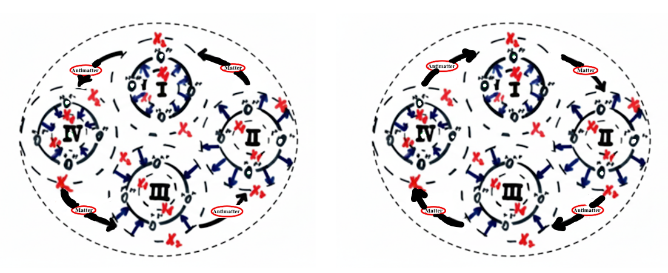
Figure 17: Schematic diagram of the entangled quartet –
If we arbitrarily choose the flow direction clockwise (right), then:
- Antimatter moves from universe IV → I and from II → III.
- Matter moves from universe I → II and from III → IV.
From the generalization of the symmetry conclusion regarding matter-antimatter and energy transfer between 'Twin Universes' (Chapter 37), a 'Symmetry of Transfer' exists across the entire 'Entangled Quartet' (see Figure 17), so that at any given time, roughly one quarter (25%) of the total mass (including energy) is present in each universe. That is, the total sum of matter, antimatter, and energy in each universe of the quartet is, on average over time, about 25% – while the remaining roughly 75% of matter, antimatter, and energy is external to the observed universe and is therefore unobservable (a ratio of 1:3). This relates to the phenomenon of self-annihilation (pure energy) when matter and antimatter meet, with its consequences discussed further in Chapter 48.
Thus, 'ToS' can provide an explanation for the order of magnitude of 'Dark Matter' in the universe. At the same time, given the current state of the expanding universe from the interior toward the 'Equilibrium Sphere', (see Chapter 11), it can also account for 'Dark Energy' (see the end of Chapter 11 – post-experiment section and Chapter 48).
Chapter 41: Color Charge / Force
The universe we inhabit (Figure 17, state I), as described in the last two chapters, is one of the 'Entangled Quartets'. Hence, the three other 'Virtual States' (II, III, IV) must balance its forces. Assuming that the force exerted by the universe is neutral (white), with no external influence on the quartet, the fictitious forces exerted by the three other virtual states must also be neutral.
Thus, we require a force to balance the 'Neutral Force' exerted by the universe – acting in three distinct ways: red, green, and blue – in such a way that their sum is always neutral, i.e., white. Hence, the Neutral 'Strong Force' (white) acting in the universe equals the total 'Color Charge Force' exerted against it.
It follows that 'ToS', in combination with the 'Twin Universes' concept, also succeeds in explaining an additional part of the standard theory of physics. For example, the framework accounts for the Strong Force (Color Charge / Force discussed in this chapter) in a fundamental way, eliminating the need to posit additional mediating particles, namely gluons, which are a central postulate of the Standard Model and remain unobserved in isolation.
Chapter 42: Spin
In Figure 17, we arbitrarily assumed the flow direction of 'Matter' and 'Antimatter' to be clockwise (right). However, for any measurement of the 'Entangled Quartet', it is likely that the flow could be clockwise or counterclockwise with equal probability (50:50) – see Figure 17. This yields two distinct, measurement-dependent possibilities for the system’s spin (±1/2).
Here, it is worth noting the insight from Chapter 4, which states that there are less-probable possibilities for the development of flow (there, the 'Wave Function'). At each point, there exists a low-probability option, which gradually increases closer to the equilibrium sphere, for the universe to 'Jump' ('Quantum Leap') to 'Any' of the other possibilities shown in Figure 17.
Thus, prior to the current universe in an 'Accelerated Expansion State' – from the interior of the 'Equilibrium Sphere' (our universe present state) – the universe could have existed in any of the other three possibilities (e.g., in a decelerated expansion), or even elsewhere within the current possibility.
It is also worth noting the significance of the 'Equilibrium Sphere Surface' as the 'Quantum Energy Level' of the 'NAVP'. Therefore, 'Quantum Energy Transitions' are possible, albeit with very low probability. Such transitions change the 'Quantum Energy Level' of the 'Equilibrium Sphere Surface', initiate motion around a new 'Equilibrium Sphere Surface', and energy is emitted/absorbed either outside the sphere (universe) or within it.
Chapter 43: The Wave Function and Other Quantities
In direct continuation of the previous chapter, the 'Wave Function' itself—similarly to the 'Up' or 'Down' States, 'Spin', 'Color, and so forth—is a 'Quantum Phenomenon' dependent on the 'Observer'.s
For an 'Observer' sufficiently distant and large enough in scale (on the order of not less than 20 magnitudes greater, as described in Chapter 38), a particle that appears classical to a nearby observer of similar scale will appear 'Quantum'.h
That is, the wave function is not absolute; it too, like the other quantities, is observer-dependent.
Hence, according to the 'Definition of Mass' based on the superposition of 'Wave Functions' (see Chapter 24), 'Mass', and 'Consequently Energy' and other related quantities, are all quantities dependent on the 'Observer’s Point of View'.
In fact, this chapter provides further proof of the invariance principle derived in Chapters 9 and 10 of Part B.
It follows that any 'Observer', in any universe—whether larger or smaller by at least 20 orders of magnitude—who is located at the same point in the 'Oscillation', will measure the same 'Speed of Light', as well as the same 'Quantum and Wave Phenomena' and the same 'Physical Constants'.
All this occurs independently 'Of the Absolute Size' of the 'Universe'.
Chapter 44: The Image of the Universe – The 'Entangled Quartet'
In Chapter 42 we examined the 'Entangled Quartet' from up close, that is, from within one of its universes.g
Another way to describe the quartet, as shown in Figure 17, is from a distant viewpoint—as a 'Wave Function Cloud' evolving over time between 'Two Boundaries', X₁ and X₂, where the surface of the 'Equilibrium Sphere' (O) represents the 'Center of Mass' of the motion (its 'Quantum Energy Level').s
Within, outside, or mixed with this 'Universal Cloud' are the three additional 'Virtual Clouds' of the Quartet—Red, Blue, and Green (see Figure 18).
Furthermore, we recall that two members of the quartet are in the 'Up' State and the other two in the 'Down' State, and that 'Two Represent Matter' while the 'Other Two Represent Antimatter'—completing the four possible combinations described in Chapter 40.

Figure 18: The image of the 'Entangled Quartet' – from a distance, the universe we inhabit (one of the quartets) appears as a single unit together with the three virtual ones.
Assuming that the universe (in orange) constitutes the 'Outer Shell' of the quartet, once a measurement or observation is made along the axis/plane 'M', and since the three other clouds of the quartet (red, blue, and green), being interwoven with one another, cannot be measured as 'Half-Clouds' or 'Half-Quarks'.H
it is reasonable to assume they will randomly align such that two of them will lie above/right of the measurement axis/plane 'M', and the third below/left—or vice versa.
If we assume—unlike the image presented in Chapter 42—that the 'Charge of the Quartet' is determined by the 'Degree of Asymmetry' in the positions of its three member clouds relative to the measurement axis/plane 'M', we will generally find that the total charge of the quartet is ±1.
Note:g
With 'Lower Probability', there 'Also Exist Cases' in 'Which All Three of the Other Clouds of the Quartet (Excluding the Outer Shell)' align on the same side of the measurement axis 'M'.J
In such cases, the 'Total Charge of the Quartet' will 'Also Be Three Times Greater' (±3) than in the more likely configuration.
Note:g
In the case of a quantum energy transition, as described at the end of Chapter 42, the 'Quantum States (Spin, Charge, Color, Etc)' of all 'All Four Members of the Entangled Quarte' will shift around the 'New Energy Level (New Equilibrium Sphere Surface').
Chapter 45: Black Hole – Singular Point or Phase Transition ?
From the very beginning of the article, we have treated the three concepts—'Near-Absolute Vacuum,' the 'Universe,' and 'Black Hole'—almost in a single breath. From Figure 18 in the previous chapter, we can see that at the center of the 'Black Hole', in a vanishingly small volume, lie the 'Center of Mass and Energy', while the 'Wave Function Clouds' of the 'Entangled Quartet' are spread around. From this, it can be inferred that a 'Space-time Singularity' exists there.
We have already mentioned several times, in previous chapters, that for a body moving near the 'Speed of Light', its 'Proper Time' contracts relative to an 'External Observer', and correspondingly, spatial distances ('Length Contraction') for the 'External Observer'.
If we also consider the principle from general relativity that acceleration is equivalent to gravity (an astronaut cannot tell whether their spaceship is accelerating or whether they are under gravitational influence), we find that a body accelerating to 'Near-Light Speed' effectively exchanges time for spatial distance, as claimed by Roger Penrose. This time–space exchange, for a body crossing the event horizon of a black hole (falling into it), can be described as a transformation of 'Spatial Coordinates' into 'Temporal Coordinates'.
Returning to the apparent singularity: as early as Chapter 12, we asked whether space could be defined, not using the conventional coordinate system of three spatial dimensions and one temporal dimension, but instead as a space with three temporal coordinates and one spatial coordinate. It appears that, at the center of the 'Black Hole', as well as in the case of acceleration to near-light speed, it is appropriate to use this three temporal coordinate system.
Using such a coordinate system, it follows that a body entering the 'Black Hole' 'Gradually Reduces', during its fall, the 'Spatial Volume' in which it is concentrated (in the three conventional spatial coordinates) to a 'Point-like Volume' (zero spatial dimensions). The loss of 'Spatial Volume' is effectively converted into a '3D Temporal Sphere with 1 Spatial Coordinate'. In this way, matter, mass, and energy disperse into a three-dimensional temporal space that expands during the fall into the 'black hole', and the 'Singularity Disappears'.
Thus, the center of the 'Black Hole' is a 'Phase Transition' point between space and time, rather than a 'Singular Point'.
Chapter 46: Elimination of the 'Gravitational Singularity' via 'ToS'
In Chapter 45, we addressed the singularity from the perspective of a 'Coordinate System Transformation' (from 'Three Spatial and One Temporal Dimension' to 'Three Temporal and One Spatial Dimension'). In this chapter, we discuss the 'Singularity' from the viewpoint of the 'ToS'.
Even if 'Quantum Fluctuations'/'Space Curvatures' existed inside the 'NAVP'/'Black Hole' (as discussed in Chapter 1 and on the later pages of the article), an 'External Observer' would be unable to observe them, as they are beyond his 'Event Horizon'. Consequently, since there are no 'Observable Quantum Fluctuations' creating the attraction as stated, there is no 'Gravitational Force' and no 'Singularity' (from the external perspective).
The only one who would be able to observe these 'Quantum Fluctuations' would be an observer living inside the 'NAVP', exactly as we observe within 'Our Own Universe', without the possibility of observing external 'Universes'/'NAVPs'.
In this way, we demonstrate that 'ToS' itself also eliminates the singularity found in 'Einstein's Equation for Gravity'. Therefore, it appears necessary to introduce a coefficient/factor to that 'Einstein's Equation'—even one that drops exponentially with proximity to the 'Schwarzschild Radius'/'Event Horizon' of the 'Black Hole'.
Chapter 47: White Hole
From the implications of the previous chapter: particles of a body falling into a 'Black Hole' disperse into a 'Temporal Sphere' of 'Vast Volume', to the point of an effectively zero average 'Time Density'. That is, in order to utilize, if at all possible, a 'wormhole/Einstein–Rosen bridge' for time travel, it would be necessary 'Time Travel' to gather all the particles of 'Matter' that 'Composed the Object', which, during the fall, dispersed through time, back into a compact 'Temporal Sphere' (with effectively zero temporal dimensions). Only then could one pass to the other side of the bridge and emerge intact, as a whole unit, with three spatial coordinates and one temporal coordinate, at 'Another Location in Space and Time', via the 'White Hole'.
In practice, it is highly doubtful that such an ability could exist, even theoretically, to collect all the information dispersed in the three-dimensional temporal sphere for its complete transfer through the bridge.
In this regard, it is worth recalling the discussion in Chapter 3 of Part B of the article, where we noted that a 'Near-Absolute Vacuum with Negligible Mass', due to the extremely large wavelength of its intrinsic frequency, has a 'Wave Function Spread' across a very large '3D Space'. Conversely, one can consider a 'Black Hole' of very high mass. Matter falling into the 'Black Hole', or even the 'Black Hole' itself, the greater its mass, the more it disperses into a large 'Temporal Volume' (a smaller 'Spatial Volume'), effectively creating a 'Effectively Creating a White Time Hole'.
Therefore, if we assume that, analogous to 'Black Holes in Space', there also exist 'Black Time Holes' (large 'Temporal Spheres' concentrated at near-zero time points), it can be inferred that the exit from such a 'Time Hole' would be through a 'White Time Hole' (an ordinary 'Black Hole')—similar to the other side of an 'Einstein–Rosen Wormhole'.
A natural question arises: are these transitions not the same as the 'Transitions Between the Twin Universes' that we 'Began Discussing Back in Chapter 33' ?
Chapter 48: The Source of 'Dark Energy'
As mentioned previously in Chapter 5, our universe is in a state of 'Expansion', from the interior of the '3D Sphere' toward the 'Equilibrium Sphere' (see Chapter 11). From this, according to Chapter 40, near the point X1 (Figure 9), the universe has lost most of its 'Antimatter' and remains composed primarily of 'Matter Particles'. Over time, more and more antimatter flows from Universe Ⅳ into our universe, while matter flows from our universe into Universe Ⅱ (Figure 17). The incoming 'Antimatter' Interacts' with the existing 'Matter', converting it into 'Pure Energy'—this is the source of 'Dark Energy'. Thus, 'Dark Energy' increases over time until the universe reaches the 'Equilibrium Sphere' ('O') while simultaneously the 'Mass' decreases. Both changes act in the same direction, accelerating the 'Expansion Rate'.
By similar reasoning, it is clear that at 'Point O', where the universe, having already lost most of its 'Matter' and continues to receive 'Antimatter' from Universe Ⅳ (Figure 17), is composed mostly of 'Pure Energy'. Consequently, its 'Mass' and 'Gravitational Force' increase, and the 'Expansion Rate' decreases accordingly.
A similar analysis can be applied to all other extreme points to determine the factors accelerating or decelerating the expansion rate. 'Mass' converts into 'Energy', accelerating the 'Expansion'; then, as 'Mass' increases at the expense of 'Energy' 'Gravitational Force' strengthens—simultaneously reducing the 'Expansion Rate'— 'cycling repeatedly'.
Chapter 49: Summary of Part E
In Chapters 37–48, we discussed the theoretical, quantum, and classical consequences of the 'ToS' combined with the 'Twin Universe Theory', on which the 'Time Machine' described in Part D is based. We obtained clear explanations for the 'Scarcity of Antimatter' in the universe, the amount of 'Dark Matter', and, ultimately, insights into the general structure of the universe, 'Black and White Holes—If They Exist'.
Finally, in the last chapter of this part, we derived the appropriate 'Conservation Law' for 'Dark Energy' which was 'Already Discussed' in Chapter 11 of Part B.
Part F: Proposed Experiment to Verify the Theory
Introduction to Part F
Chronologically, this experiment was written prior to Parts D and E of the paper (the theory based on the 'ToS'). These later parts were eventually found to contradict the method proposed here for measuring the temporal variation in the speed of light.
This contradiction, of course, arises from the fact that if the 'Entangled Quartet Theory' is indeed correct—as distinct from the ToS' itself—it 'Necessarily Follows' that we cannot separate the members of the 'Entangled Quartet'. Therefore, the 'Mass' measured will be the combined mass of all four, which, unlike the 'Mass' of each individual universe, will remain 'Constant Over Time'. Thus, the 'Indirect Method of Measurement' proposed in this experiment—to determine changes in the 'Speed of Light', over time, through 'Mass Variations' (Chapter 52)—essentially fails.
Nevertheless, and despite the aforementioned contradiction, I chose to keep this proposed experiment as part of the complete 'Conceptual Development' of the paper—perhaps also in the hope that one day it will be possible to find a way to measure changes in the speed of light and mass for each of the four entangled universes separately.
.(A 'Revised Experiment', designed to measure the 'Rate of Change in the Speed of Light' over an 'Extended Period of Time', will be presented later, toward the end of this part)
Chapter 50: A Brief Summary of the Paper
In part B of the paper (Chapters 1–13), we found that space curvature, gravitational force, and, in fact, a 'Unified Theory of the Four Known Fundamental Forces of Nature' (Electromagnetic, Gravitational, strong nuclear, and weak nuclear) all emerge—through the synthesis arising from quantum theory—as a direct consequence of the natural assumption that the universe is composed of countless 'NAVPs'.j
(Later, toward the end of part C (Chapters 26–29), we understood that these points are, in a sense, connected to the surrounding space at their centers)
Continuing within part B, we saw that the 'Harmonic Oscillation Characteristics' of the 'NAVPs' around their 'Equilibrium'—at the 'Oscillation Speed' (C) the 'Maximum Possible Velocity in Nature', which 'Itself Varies Over Time' between 0 at the extremes and almost infinitely high at the center (the surface of the equilibrium sphere)—define 'Matter', 'Antimatter' and 'Dark Matter and Energy' as we know them.
We also recalled from 'Relativity Theory' that as an object’s velocity approaches the 'Speed of Light,' its 'Mass' increases and its 'Proper Time' slows down (the well-known 'Twin Paradox').
In addition, we referred to the well-known relation E=MC2 and to the 'Principle of Invariance of the Laws of Physics', independent of the universe’s relative scale.
We then attempted—apparently without great success—to propose a thought experiment for measuring the temporal change in the speed of light since the birth of the universe, through the present and into the future.
However, what we did obtain was a partial explanation for the extraordinarily high, previously unexplained energy observed in quasars.
In part C (Chapters 14–32), we shifted the 'Frame of Reference'—the 'Origin of Coordinates'—from a 'Hidden Coordinate System' centered on the 'Center of Mass', to a more natural system whose 'Origin' lies at the 'NAVPs'.j
We showed that, physically, both frames of reference are equivalent, so that reality can be described from either viewpoint independently—or even simultaneously.
Later, by redefining the concept of mass and analyzing the motion of the center of mass, we found that this additional point of view clarifies many other phenomena, such as: the 'Constancy of the Speed of Light' in all directions, 'Heisenberg’s Uncertainty Principle' 'Photons' 'Superconductivity', 'Casimir Effect' and so forth.
Finally, in the last chapter of this part, we briefly discussed wave propagation in space from the perspective of the new coordinate system.
In part D (Chapters 33–36), building on the knowledge accumulated earlier, we proposed a theoretical framework for constructing a 'Time Machine'—including a numerical example—and a partial examination of its theoretical implications.
In part E (Chapters 37–49), based on the 'ToS' and the 'Twin Universes Theory'—upon which the 'Time Machine' of Part D relies—we obtained compelling explanations for the observed 'Scarcity of Antimatter' in the universe, and for the quantities of 'Dark Matter' and 'Dark Energy Within It'.
From these considerations, we also derived general insights regarding the structure of the universe, and the nature of black and white holes, to the extent that they exist.
After all of these (the first through last part of the paper), it seems that we are still left with the greatest open question of all:
Based on everything discussed so far—how, and whether, it is possible to prove that the 'Speed of Light', as predicted by the theory, indeed changes over time.
Chapter 51: The Challenges Ahead
- It seems that no direct method currently exists—or at least none has been discovered so far—for measuring long-term 'Variations in the Speed of Light'.
- Even if such a method were found, measuring 'Variations in the Speed of Light' would require observations extending over an immensely long period—billions, or at the very least, hundreds of millions of years.
Chapter 52: Solving the First Challenge (Indirect Measurement)
To address the first challenge—and since it is quite evident that directly measuring long-term variations in the speed of light would be practically impossible—we shall propose an indirect approach.
For this indirect measurement, we turn to the well-known equation E=MC2, and argue that measuring 'Mass Variations' of a point of 'NAVP' (or even if it possesses some other finite mass), under the assumption that its 'Total Energy Variations Over Time are Negligible' (i.e., a 'Closed System'), is in fact an 'Indirect Yet Equivalent Measurement'.
That is to 'Say': as 'Implied by the Equation', and assuming that the energy variations over time are indeed negligible, any change in the 'Speed of Light' (C) is inversely proportional to the square root of the change in 'Mass' (M).
Thus, to 'Measure the Variation in the Speed of Light'—and thereby test the theory—it is sufficient, in practice, to measure 'Long-Term Mass Variations'.
Chapter 53: Solving the Second Challenge (Time Dilation)
We are left with the second difficulty, which at first glance appears even greater than the first.
As known from the theory of relativity, a body moving at a velocity approaching the the 'Speed of Light' 'Experiences an Increase in Mass and a Slowing of Its Proper Time'. In other words: 'The greater the mass of a body, the more slowly its proper time flows'.
Conversely, time as measured by an 'External Observer' flows much faster than the 'Proper Time' experienced by an 'Observer' located on the 'Massive Body'.
Thus, depending on the body’s mass—for instance—100 million or even a billion years that pass for us could correspond to only half a year for an observer residing on the mass itself.
Therefore, when we measure 'Mass Variations' in the 'Body’s Mass' over a half-year period, we are, according to the 'Principle of Invariance', effectively measuring mass changes that, in our own time units, 'Correspond to a Much Longer Duration'—the time that would pass for the external observer.
Explanation of the invariance principle:
In our example, 'Variations of X%' in the 'Body’s Mass' and in the universe’s mass (or in the 'Speed of Light'), occurring over roughly half a year for the 'Observer' on the 'Mass', may correspond to similar variations taking place over a span of 100 million or even a billion years for us—depending on the 'Mass Ratio' involved.
Chapter 54: The Experiment
All that remains is to find a body of sufficiently 'High Mass'—one for which the 'Difference in Time Flow' between an 'Observer Located on the Mass' and 'One Located Outside' would be as large as possible—on which such a measurement could be performed.
The most natural candidate for this purpose, quite evidently, is a 'Black Hole'.
For the measurement, we may select either a single 'Black Hole' or a 'Binary Star System' in 'Which One of the Components Is an Invisible Black Hole', and propose the following experimental observations:
- 'I'Indirect measurement' of 'Mass Variations' of the 'Black Hole', by monitoring, over a period of roughly half a year, the changes in the bending intensity of light rays from a distant star passing near it (similarly to the historical experiment demonstrating the deflection of starlight by the Sun’s mass in support of general relativity).
- Alternatively, in a 'Binary Star System' in 'Which One Component Is a Black Hole', we may 'Directly Measure the Effect of Mass Variations' in the 'Black Hole’s Mass'—again over a period of roughly half a year—on its 'Companion Star'.
Chapter 55: Experimental ResultS
If, over time, measurable 'Variations'—whether increases or decreases—in 'Mass' are indeed observed, this would imply that the 'Speed of Light' (C) (or the 'Oscillation Rate' of the 'Black Hole') also varies with time, exactly as predicted by the theory.
As stated earlier, the variation in the speed of light should be inversely proportional to the square root of the variation in mass.
Notes:
- The 'Variation in the Speed of Light' may correspond to either an 'Increase or a Decrease', depending on the 'Oscillation’s Position Relative to the Equilibrium Point':
– When the oscillation moves toward the equilibrium point, the speed of light increases (mass decreases).L
– When the oscillation passes beyond the equilibrium point—'Either Inward or Outward Relative to the Equilibrium Sphere'—the 'Speed of Light' decreases (mass increases). - A possible outcome: It may well be that some, or even a significant portion, of pulsar stars—which 'Exhibit Periodic Variations in Their Intensity'—could be explained by fluctuations in the mass of a neighboring black hole or another massive, unseen companion.
Summary of Part F (New Proposed Experiment to Verify the Theory)
In summary, the 'Proposed Experiment' section was intended to test the theory—and a few years after its completion—I found it appropriate to add the following note:
After being asked by many readers to propose a possible experiment for measuring the rate of change in the 'Speed of Light' over time, and Since the Proposed Experiment in the begining of This Section was ultimately found to be inconsistent (as discussed in the introduction to this part), a New and Corrected Experimental Proposal was written in early 2023.
This 'Updated Version', 'Based on the End of Chapter 11 in Part B of the Paper', can be found in the linked materials, including the updated experimental proposal (optical).
/https://www.shimony.co.il/e-v-experiment-proposal-nov-2025
Epilogue
This paper, which began with the modest goal of seeking a possible path toward 'Unifying the Force of Gravity with the Other Known Fundamental Forces of Nature' (Chapter 1), has gradually evolved into a quantum (geometrical) theory of gravitation.
Along the way, the theory continued to evolve, offering explanations (sub-theories based on the 'ToS') for many additional phenomena, as well as a proposed experiment for its verification.
I believe that should the 'New Proposed Experiment to Verify the Theory' succeed in finding the exact Ct distribution function over time, all other constant – such as the Gravitational Constant (G), cosmology Constant (Λ), the Strong Force coupling constant – as well as microphysical parameters like Schwarzschild radius, atomic and nuclear size, will be defined purely as a function of the measured Ct'. This establishes the mechanism for observing the universe's evolution through the measurement of microphysical constants across cosmic time, thereby providing a direct experimental path to validate the theory.
Moreover, I believe that, with full mathematical precision (including time depended), this theory will astonish us still further:J
it may resolve many of the remaining mysteries of modern physics, and—as with every new scientific theory—it will undoubtedly raise new questions of its own, awaiting future exploration and understanding.
Eran Shimony, 2025 ©
English translation based on the original Hebrew version of the 'Theory of Spheres' (ToS) (2017).
All rights reserved by the author.
To the beginning of the article
Related Papers in the Theory of Spheres Series:
'Theory of Spheres – experiment-proposal'
'Theory of Spheres – Part III'
'Theory of Spheres – Part III(a)'
'Theory of Spheres – Part Ⅳ'